Kaggle: Prime Travelling Santa 2018 - MIP

First of all I want to say sorry for not writing in the last couple of months. University is stressful, I think that should be a good enough excuse :D Anyway I don't get paid for it so I don't have to say sorry :P

Okay let's get back to some Julia code and some optimization in 2019. I got my second silver medal at Kaggle now and this is the first post about achieving that. During the last Christmas break there was another optimization challenge which is always my favorite as it is an optimization challenge every year.

This blog post is about a MIP version I tried to solve part of the problem and even though some parts didn't work out well and in the end we probably wouldn't have need it at all if we had something much better, it might still be interesting for some of you. I completely coded this part so I'll start with blogging about it. (This time I was in a team at Kaggle ;) ) My next post will be on kopt which a teammate started and I improved on it.

Okay enough small talk. Let's start.

The challenge

I should first introduce you to the kaggle challenge: It was basically a big TSP problem with roughly 200,000 cities. The goal was to find the shortest path for rudolph, the reindeer, starting from the north pole visiting every city once and then back to the north pole. That wouldn't really be the style of a real kaggle challenge so there was an extra. Every tenth step costs 10% extra if the starting point of this step is not a prime city, a city where the city id is a prime number. At first glance: This means that the score is roughly 1% different than a normal TSP (if you only solve the TSP) as there are about 20,000 prime numbers below 200,000.

Visualization

You know me so we first start with a proper visualization of the challenge. First of all we download all the files from kaggle and then I change the cities.csv to include all the prime cities saving it in cities_p.csv to not calculate the prime cities every time.

using CSV, DataFrames, Plots

cities_csv = CSV.read("cities_p.csv");

gr()
prime_idx = findall(cities_csv[:prime] .== true);
nprime_idx = findall(cities_csv[:prime] .!= true);
width = 5100
height = 3400

plot(cities_csv[:X][prime_idx], cities_csv[:Y][prime_idx], markersize=1, seriestype=:scatter,
    size = (width, height), label="", color=:orange, axis=false)
plot!(cities_csv[:X][nprime_idx], cities_csv[:Y][nprime_idx], markersize=1, seriestype=:scatter,
    size = (width, height), label="", color=:black, axis=false)
png("blog")

which produces this image: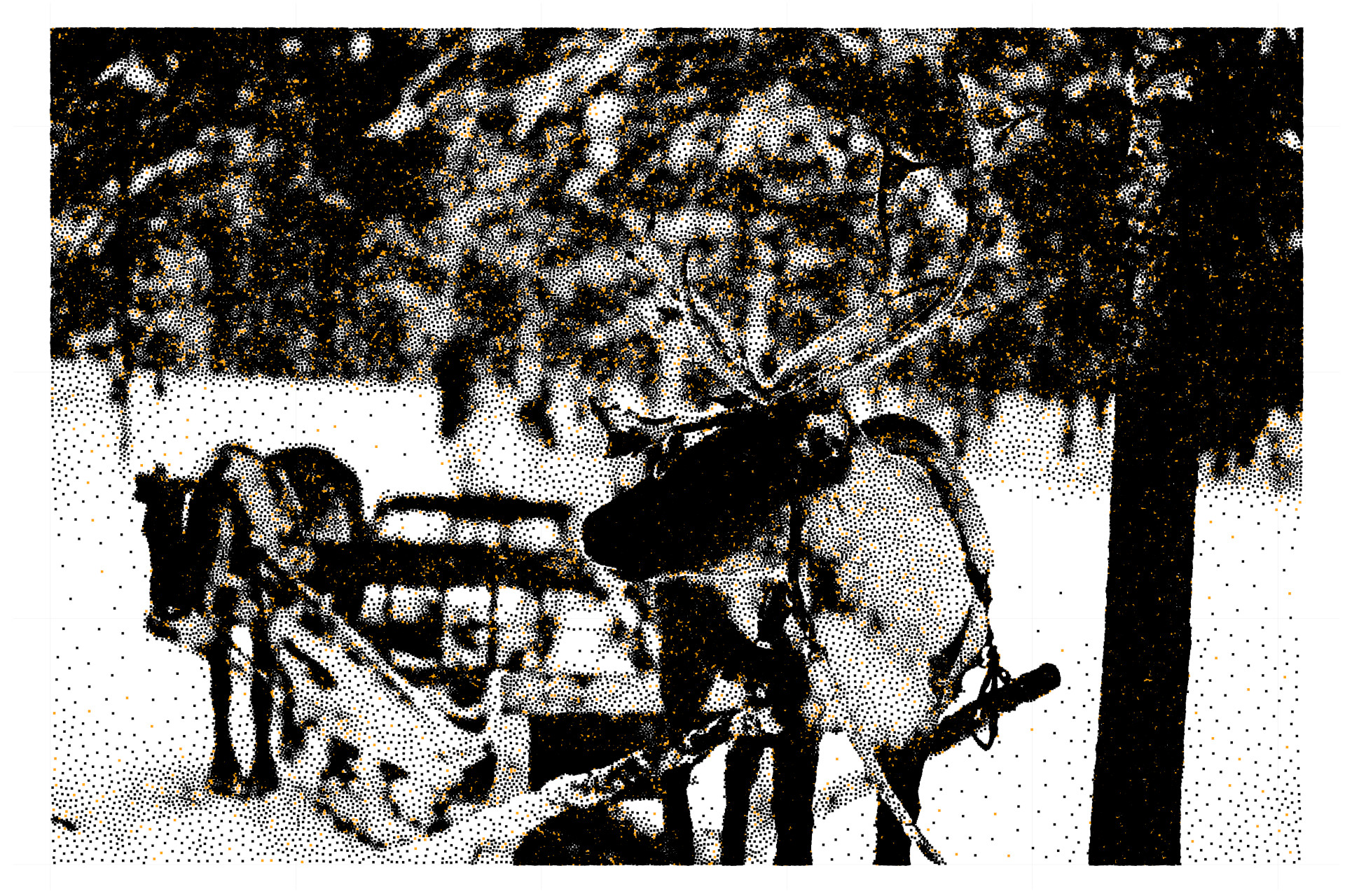

If you didn't read the code: the orange cities are the prime cities and the black pixels are the "normal" cities.

and we can calculate how many cities there are and how many are primes:

#cities: 197769
#primes: 17802

which means that about 9% are prime and with our 10% extra costs the prime cities are not that important so at first glance it seems to be about a normal TSP.

Therefore it seems natural to get a good TSP solution first and improve on that but I was a little lazy so I just used a kernel solution that someone had posted: this one by @blacksix

Which uses the famous concorde solver, the best TSP solver out there. It runs for 5 minutes so nobody can expect that much but it's a good starting point for us. Later we can think about a better initial solution.

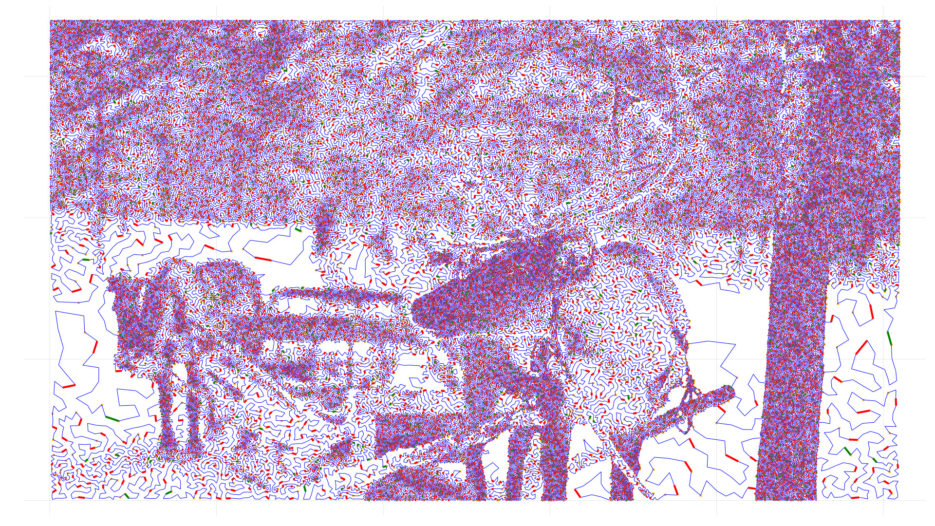
As you can see it is a wonderful picture and the reindeer you have imagined before is perfectly visible. This is not only a blog about optimization or MIP or whatever but mainly about opensourcing ideas and code therefore a short explanation of how I visualized it using Julia.

First we create a Cities struct where we save the position of the city and not prime as a vector. Yeah I could have saved prime here as well. Don't ask!

mutable struct Cities
    xy :: Array{Float64,2}
    nprimes :: Vector{Float64}
end

Now reading the submission file:

temp_df = CSV.read("submissions/5min_concorde.csv");
subm_path = temp_df[:Path];

and check whether it is a valid path by checking whether every city is in it:

test_sp = sort(subm_path)
@assert test_sp[2:end] == collect(0:197768)

Construct a vector with every tenth edge and add one to the 0 indexed based subm_path as we are coding in Julia...

tenth_full = [(i % 10) == 0 for i in 1:length(subm_path)-1]
subm_path .+= 1

Also saving the position and the non primes to the struct we created:

xy_cities   = zeros(size(cities_csv)[1],2)
xy_cities[:,1] = cities_csv[:X] 
xy_cities[:,2] = cities_csv[:Y]
cities = Cities(xy_cities, cities_csv[:nprime])

Constructing a vector where we save whether it is the tenth edge and not coming from a prime based on our submission path and plot the prime cities as before.

tenth_and_noprime = cities.nprimes[subm_path] .* tenth_full
plot(cities_csv[:X][prime_idx], cities_csv[:Y][prime_idx], markersize=1, seriestype=:scatter,
    size = (width, height), label="", color=:orange, axis=false)

We want to plot everything in one go (this can be used for making an animation as you see later)

k = 1
step_length = length(subm_path)

Now we have red edges, green edges and normal/black edges. The red edges are edges where we have 10% extra costs, the green where we avoided them and the normal edges are normal ;).

red_tenth_x = Plots.Segments()
red_tenth_y = Plots.Segments()             
green_tenth_x = Plots.Segments()
green_tenth_y = Plots.Segments()   
normal_x = Plots.Segments()
normal_y = Plots.Segments()

Now we want to fill this Segments which basically just means that we can plot a segment later in one go. If you fill a normal array everything will be connected like the end of a green edge with the start of the next green edge which would be wrong.

for i=k:k+step_length
    if i+1 > length(subm_path)
        break
    end
    if tenth_and_noprime[i] == 1
       push!(red_tenth_x, cities_csv[:X][subm_path[i:i+1]])
       push!(red_tenth_y, cities_csv[:Y][subm_path[i:i+1]])
    elseif tenth_full[i]
       push!(green_tenth_x, cities_csv[:X][subm_path[i:i+1]])
       push!(green_tenth_y, cities_csv[:Y][subm_path[i:i+1]])               
    else
        push!(normal_x, cities_csv[:X][subm_path[i:i+1]])
        push!(normal_y, cities_csv[:Y][subm_path[i:i+1]]) 
    end
end

Here the normal edges are added one by one which could be improved but I didn't care.

And just plot it. Btw plot! means that you add it to the previous plot.

plot!(normal_x.pts, normal_y.pts, linewidth=1, 
      seriestype=:path,size = (width, height), color = :blue, label="", axis=false, 
      legend=false, colorbar=false)
plot!(red_tenth_x.pts, red_tenth_y.pts, linewidth=4, 
      seriestype=:path,size = (width, height), color = :red, label="", axis=false, 
      legend=false, colorbar=false)
plot!(green_tenth_x.pts, green_tenth_y.pts, linewidth=4, 
      seriestype=:path,size = (width, height), color = :green, label="", axis=false, 
      legend=false, colorbar=false)
savefig("latest.png")

Okay that is everything for the visualization part for now. Some additional information we can obtain are:

Normal distance: 1,504,825.37
Extra: 13,654.31
Extra #: 17,982
Tenth #: 19,776
Zero Extras #: 1,794
Santa score: 1,518,479.69

which you can easily calculate. It means that our current normal TSP score is 1,504,825.37 and we have extra costs of ~13,000 and avoid extra costs ~1,800 times by chance as we didn't optimize that yet.

MIP No. 1

I was wondering how to write a MIP that solves the problem to an optimal level for smaller versions. I didn't come up with a super nice solution but we can have a look how much it is able to improve our current solution. Hope you have read my MIP TSP article.

The idea is pretty much the same but we need to have the position of each city in the path to calculate the precise santa score. My formulation in Julia JuMP code:

Creating the model as usual:

m = Model(solver=CbcSolver(OutputFlag=0))

Create variables for the edge. One edge is characterized by the start city, the end city of the edge and the position of the edge. Which results in \(N^3\) edges which is obviously bad but simple :D

@variable(m, x[1:N,1:N,1:N], Bin)

We define our objective by minimizing the distance and we have extras defined as 1.0 or 1.1 based on something like tenth_and_noprime.

@objective(m, Min, sum(x[i,j,s]*dists[i,j]*extras[i,s] for i=1:N,j=1:N,s=1:N));

A city is not allowed to connect to itself, each step is allowed only once which means we can't have two edges which are both edge No. 1 to avoid the extra costs.

@constraint(m, notself[i=1:N], sum(x[i,i,1:N]) == 0);
@constraint(m, eachsteponce[s=1:N], sum(x[1:N,1:N,s]) == 1);

and each city must have an outgoing and one incoming edge to form a cycle.

@constraint(m, oneout[i=1:N], sum(x[i,1:N,1:N]) == 1);
@constraint(m, onein[j=1:N], sum(x[1:N,j,1:N]) == 1);

now if we have and edge from i to j in step s we need an edge from j in the next step:

for s=1:N-1
    for i=1:N,j=1:N
        if i != j
            @constraint(m, x[i,j,s] <= sum(x[j,1:N,s+1]));
        end
    end
end

And the tour should start at the first point in our array and end in the last, so that we later can still combine the parts easily.

@constraint(m, sum(x[1,1:N,1]) == 1);
@constraint(m, sum(x[1:N,N,N-1]) == 1);

I optimized every fifth step with N = 20 for ~3 hours (until roughly 1/4 of the path) and the resulting score was about 30 points better. Just wanted to show that it is not very effective. My goal was to increase the N to something like 200 for a bigger impact. For testing purposes I tried this with Gurobi and Cbc where later I only used Cbc as Gurobi is a commercial software.

Some timings for various N.

N	Cbc	Gurobi
20	12s	0.5s
30	180s	10s
40	-	50s

for N=40 and Cbc I was just not patient enough... but you can clearly see that it is not really worth it to increase it to N=200 or something similar even when using Gurobi. We would need \(200^3 = 8,000,000\) variables which is quite big. Additionally Gurobi is much better probably because my formulation can be simplified and Gurobi has just better techniques ;)

MIP No. 2

There are some other techniques of reformulating the problem into a more general TSP form as pointed out by some people in various Kaggle discussions but they didn't seem to have much luck and I probably just wanted to try something else... At the end it turned out by having a look at the winning solutions that MIP or similar local optimization techniques didn't work out. If you're still interested:

The idea is pretty simple and I'll just make our repository public then you can have a look at the source code. It's not well documented currently :/ but this should help you to read it.

We solve a TSP with the same code as shown in my post about MIP and TSP but we use the better formulation where an edge is only represented in one direction so 1->2 is the same as 2->1 therefore we only have 1->2 as an option. This is explained in the MINLP TSP version here. We check whether this is an improvement of our current solution, based on the actual santa score, which is normally not the case and then resolve it by disallowing the cycles we have already found. We basically solve the k shortest TSP problem and check every time whether the santa score improved. We also can approximate the minimal extra costs in this subpath as we know how many primes there are and check whether that is enough to avoid every penalty and otherwise we compute the minimal distance in this city cloud and multiply it with the minimal amount of penalties and add it to the shortest path. This is an upper bound for our normal TSP score to achieve a better santa score.

I've run this on the same initial solution for about 3 hours as well and got an improvement of about ~19 per hour. This run would take ~35hours on 6 cores which would result in >600 points which is way better than the one with N=20. I didn't use a stride here so afterwards we can run a second run which starts at the half of each current block which probably would result in an increase of ~200 additional points.

In general I want to point out that both of these approaches can be faster by doing them in parallel as it is a local approach.

This video shows you our final tour after using a better starting solution and kopt and the MIP local search as described above:

In the next post I'll explain our kopt implementation.

Please have a look at our code at:

GitHub

If you enjoy the blog in general please consider a donation via Patreon. You can read my posts earlier than everyone else and keep this blog running.

Want to be updated? Consider subscribing and receiving a mail whenever a new post comes out.

Enter your email

Powered by Buttondown.