Benchmarking and Profiling Julia Code
Creation date: 2021-03-21

Welcome back to a new part in our Julia basics series where I explain some basic functionality of the Julia programming language.
In this post I'll explain various possibilities to find slow code in your project. You might have already researched the Julia documentation and other websites regarding this. Often they will do this using small code examples which can be easily analyzed and are helpful for training. Nevertheless I feel some things can only be seen when having a look at bigger packages.
Well you're here so I assume that small code examples didn't help you out too much. You might want to infiltrate some bigger projects of your own. Then you're at the right place.
Let's get started with a small code example as well 😄 and use it for the most part of this post. However, in the last part I'll be having a look at my own package which implements a constraint solver, see: ConstraintSolver . You can also see quite a few posts about that project on this blog when you check out the sidebar on the left.
I know that this mathematical optimization thing can be a bit overwhelming but I assure you that I will not talk about that project here. I'll simply use it as a codebase to analyze the performance and the first 90% of the post are about a very small code example. 😉
Even though that is the case we'll learn about the tools to keep manageable for bigger code bases whereas the Julia documentation is a bit too fine detailed for me and provides often a performance profile that is longer than the code which feels daunting.
One last thing before we dive into it. I've recently started to create an email subscription list to send you the newest posts. It's often a bit hard to keep track of new posts when they don't get posted on a regular schedule. So if you want to get informed about new posts roughly twice a month consider subscribing to the list for free. Thanks a lot!
Free Patreon newsletterThe post is split into some sections to make it easier for you to jump around as the post is a bit long. 😉 We'll start with having a look at BenchmarkTools first to understand basic time measurement of functions and get an overall feeling of the speed. This will include some things to consider when timing functions in Julia as one has to be aware of compiling time.
Afterwards we will have a look at memory allocations in particular as this is often a good place to start with when trying to speed up code. For both these sections we will use a small julia script as an example to make sure we understand everything for a small enough function.
The final step will be to have a look at the ConstraintSolver codebase to find a particular section of the code that is slowing down the solver.
A small code example
Let's assume we want to find all prime numbers up to a number.
function get_primes(to)
    possible_primes = collect(2:to)
    # iterate over the primes and remove multiples
    i = 1
    while i <= length(possible_primes)
        prime = possible_primes[i]
        possible_primes = filter(n->n <= prime || n % prime != 0, possible_primes)
        i += 1
    end
    return possible_primes
end

# create a list of numbers from 2:100
possible_primes = get_primes(100)
Benchmarking
Let's don't have a look at the code from above in detail here and just figure out how fast it is for different input sizes.
It's possible to just use the macro @time for this and run:
@time get_primes(100)to see that it takes 0.00....X seconds so one might consider that fast 😄 The problem with using the @time macro is that it can include compile time if it's the first time we call that function. Additionally it calls the function once only so it can depend on a lot of other variables like how busy is your CPU because you currently watch a YouTube video?
For this you want to run the function several times and get some statistics like median and mean running time. Therefore we want to use the BenchmarkTools package.
In one of the earlier posts about packages I've explained how to install packages and environments and stuff like that. If you haven't already you can install the package by typing ] add BenchmarkTools into your REPL.
Perfect! Now let's do some measurements for prime numbers up to 100, 1,000, 100,000, 1,000,000.
julia> using BenchmarkTools
julia> @benchmark get_primes(100)
BenchmarkTools.Trial:
  memory estimate:  8.80 KiB
  allocs estimate:  26
  --------------
  minimum time:     2.165 μs (0.00% GC)
  median time:      2.592 μs (0.00% GC)
  mean time:        3.064 μs (3.01% GC)
  maximum time:     85.641 μs (96.03% GC)
  --------------
  samples:          10000
  evals/sample:     9
I think it might be hard to get a feeling for whether this is fast or not so let's test it for bigger numbers. We use the macro @btime for this to get only the minimum elapsed time.
for n in [1000, 10000, 100000, 300000]
    println("n: $n")
    @btime get_primes($n)
end
Here we use $ to interpolate the variable inside the @btime macro.
n: 1000
  71.448 μs (169 allocations: 264.69 KiB)
n: 10000
  3.926 ms (1241 allocations: 11.95 MiB)
n: 100000
  235.344 ms (19190 allocations: 705.86 MiB)
n: 300000
  1.698 s (52000 allocations: 5.05 GiB)
I would say the scaling of this is quite bad. Certainly we don't want to wait for more than a second to get the prime numbers up to a 300 thousand.
As we have only a single function we are more or less done with the benchmarking section for this code. You might be interested in plotting the timing.
Actually yeah why not... A little graph is always nice and we can learn to retrieve the timing information from BenchmarkTools .
Installing Plots with ] add Plots
using Plots

xs = Float64[]
ys = Float64[]
for n in range(100, stop=50000, length=20)
    println("n: $n")
    t = @benchmark get_primes($n) seconds=1
    push!(xs, n)
    # convert from nano seconds to seconds
    push!(ys, minimum(t).time / 10^9)
end
plot(xs, ys, legend=:topleft, label="Calculating prime numbers", xaxis="Primes up to", yaxis="Time in seconds")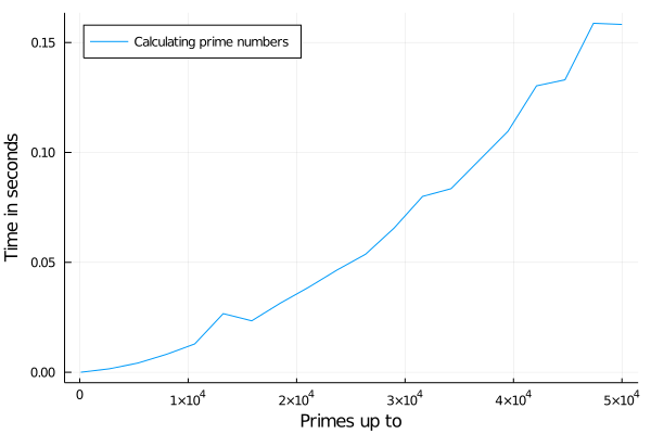
You can of course experiment a bit with logarithmic scales or something and more data but I think we have a rough understanding of how it scales now 😉
Memory Allocations
In this section we will try to understand memory allocations of the above mentioned prime code.
You might have realized that @btime and @benchmark also show the memory consumption.
n: 1000
  71.448 μs (169 allocations: 264.69 KiB)
n: 10000
  3.926 ms (1241 allocations: 11.95 MiB)
n: 100000
  235.344 ms (19190 allocations: 705.86 MiB)
n: 300000
  1.698 s (52000 allocations: 5.05 GiB)
It certainly doesn't take 5GiB to store the prime numbers from 2 to 300,000, right? I mean we don't even need that much memory to store all the numbers from 2 to 300,000 which should probably be more or less our limit.
julia> sizeof(collect(2:300000))
799992
based on wolfram alpha this is 2399992 bytes in MiB => 2.29MiB 😄
Okay so without diving into the code just yet as it's probably not that hard to see why we need so much memory... Let's create a file for that program primes.jl and then start a julia session with julia --track-allocation=user.
Then use:
include("primes.jl")
get_primes(100000)
and close the julia session.
This generates a .mem file in the directory where we creates primes.jl Unfortunately this is the output for it:
- function get_primes(to)
800080     possible_primes = collect(2:to)
    -     # iterate over the primes and remove multiples
    -     i = 1
    0     while i <= length(possible_primes)
    0         prime = possible_primes[i]
    0         possible_primes = filter(n->n <= prime || n % prime != 0, possible_primes)
    0         i += 1
    -     end
    0     return possible_primes
    - end
Which is clearly not the correct result as we had more memory allocations.
It was actually a bit unexpected for me to see this as it's normally my goto tool for having a look at memory allocations.
Fortunately there are other ways to track this which we will cover now 😉
TimerOutputs is a package that times specified parts of a function and combines their running time when allocations happen in a loop.
One drawback of this is that you need to change the code a bit to tell TimerOutputs where we want to measure time and allocations.
I have changed it to:
using TimerOutputs
tmr = TimerOutput()

function get_primes(to)
    @timeit tmr "collect" possible_primes = collect(2:to)
    # iterate over the primes and remove multiples
    i = 1
    @timeit tmr "loop" begin
        while i <= length(possible_primes)
            prime = possible_primes[i]
            possible_primes = filter(n->n <= prime || n % prime != 0, possible_primes)
            i += 1
        end
    end
    return possible_primes
end
and after running get_primes(100000)
we can get the results:
julia> show(tmr)
 ──────────────────────────────────────────────────────────────────
                           Time                   Allocations
                   ──────────────────────   ───────────────────────
 Tot / % measured:      11.1s / 2.58%            783MiB / 90.1%

 Section   ncalls     time   %tot     avg     alloc   %tot      avg
 ──────────────────────────────────────────────────────────────────
 loop           1    280ms  97.9%   280ms    705MiB  100%    705MiB
 collect        1   5.97ms  2.09%  5.97ms    790KiB  0.11%   790KiB
 ──────────────────────────────────────────────────────────────────
Here one can see that collect is not the main memory allocator in our code. It lies somewhere in our loop.
We could specify more @timeit macros inside of our code like:
function get_primes(to)
    @timeit tmr "collect" possible_primes = collect(2:to)
    # iterate over the primes and remove multiples
    i = 1
    @timeit tmr "loop" begin
        while i <= length(possible_primes)
            prime = possible_primes[i]
            @timeit tmr "filter" possible_primes = filter(n->n <= prime || n % prime != 0, possible_primes)
            i += 1
        end
    end
    return possible_primes
end
and get:
julia> show(tmr)
 ───────────────────────────────────────────────────────────────────
                            Time                   Allocations
                    ──────────────────────   ───────────────────────
  Tot / % measured:      6.62s / 4.26%            711MiB / 99.3%

 Section    ncalls     time   %tot     avg     alloc   %tot      avg
 ───────────────────────────────────────────────────────────────────
 loop            1    282ms   100%   282ms    706MiB  100%    706MiB
   filter    9.59k    268ms  95.1%  27.9μs    705MiB  100%   75.3KiB
 collect         1   73.9μs  0.03%  73.9μs    781KiB  0.11%   781KiB
 ───────────────────────────────────────────────────────────────────
This also shows how often the filter is called and we can indeed see that filter is responsible for the memory allocations.
@timeit itself has some running time and memory allocation overhead but it gives us a good idea of where we need to have a deeper lookEven though this post is about profiling I want to point out that one can use filter! with the ! to update the collection inplace. Currently we create a new vector every time.
using TimerOutputs
tmr = TimerOutput()

function get_primes(to)
    @timeit tmr "collect" possible_primes = collect(2:to)
    # iterate over the primes and remove multiples
    i = 1
    @timeit tmr "loop" begin
        while i <= length(possible_primes)
            prime = possible_primes[i]
            @timeit tmr "filter!"  possible_primes = filter!(n->n <= prime || n % prime != 0, possible_primes)
            i += 1
        end
    end
    return possible_primes
end
with the TimerOutputs table:
julia> show(tmr)
 ────────────────────────────────────────────────────────────────────
                             Time                   Allocations
                     ──────────────────────   ───────────────────────
  Tot / % measured:       6.06s / 3.53%           5.31MiB / 22.5%

 Section     ncalls     time   %tot     avg     alloc   %tot      avg
 ────────────────────────────────────────────────────────────────────
 loop             1    214ms   100%   214ms    442KiB  36.2%   442KiB
   filter!    9.59k    201ms  94.1%  21.0μs    300KiB  24.5%    32.0B
 collect          1   73.9μs  0.03%  73.9μs    781KiB  63.8%   781KiB
 ────────────────────────────────────────────────────────────────────
As mentioned above for small allocations and times the overhead of @timeit can come into play. We can verify easily with BenchmarkTools that filter! actually doesn't have any allocations.
Before we continue with the profiling section and the bigger codebase you might want to experiment a bit with the code and see how much faster you can make the code 😉
using Plots
xs = Float64[]
ys_slow = Float64[]
ys_faster = Float64[]
for n in range(100, stop=50000, length=20)
println("n: $n")
push!(xs, n)
t_slow = @benchmark get_primes_not_inplace($n) seconds=1
t_faster = @benchmark get_primes($n) seconds=1
# convert from nano seconds to seconds
push!(ys_slow, minimum(t_slow).time / 10^9)
push!(ys_faster, minimum(t_faster).time / 10^9)
end
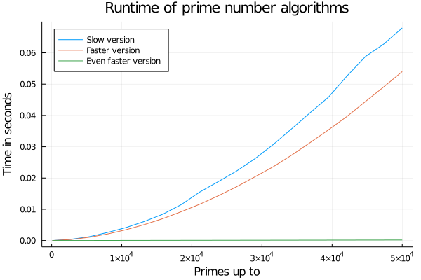
plot(;title="Runtime of prime number algorithms", legend=:topleft, xaxis="Primes up to", yaxis="Time in seconds")
plot!(xs, ys_slow, label="Slow version")
plot!(xs, ys_faster, label="Faster version")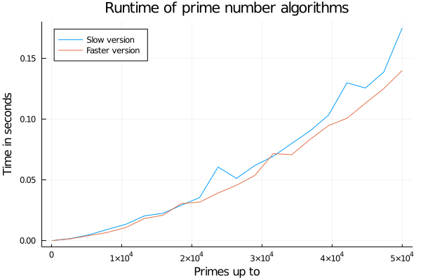
We got a bit faster and reduced memory consumption. In the last section we will have a short look at the flamegraph of this prime function and I'll give one other faster way of computing the primes.
Profiling
We had a look at basic benchmarking where we get the running time of the function we call. How about getting this information for all functions inside the main function and recursively apply that down to the very basic functions like == and +?
Profiling is a bit like that but does not necessarily give information about the exact running time of these functions. I would say it's a bit more vague but gives a very nice overview of where your code takes the most amount of time.
Let's start with our in-place version of the prime function.
For reference:
function get_primes(to)
    possible_primes = collect(2:to)
    # iterate over the primes and remove multiples
    i = 1
    while i <= length(possible_primes)
        prime = possible_primes[i]
        possible_primes = filter!(n->n <= prime || n % prime != 0, possible_primes)
        i += 1
    end
    return possible_primes
end
For profiling we need another two packages where one (Profile) is part of the standard library so we don't need to run ] add for that. The other is PProf which visualizes the profiling data and needs to be installed.
We write:
using Profile, PProf

get_primes(100000);
@profile get_primes(100000)
pprof(;webport=58699)
You can then click on the link to "http://localhost:58699" which will show a call graph. I don't like the graph representation that much which is the reason why I often switch to
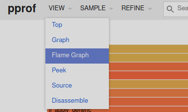
This will then show something like this (scroll down a bit 😉)
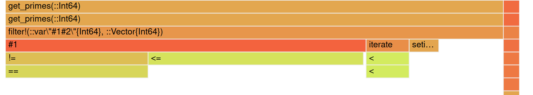
For our current implementation this is quite simple: We have the get_primes function and beneath that the filter! function. The flamegraph has those blocks which have a width that is representing the time spent in that function. Blocks below other blocks are inner functions.
Two important things to note:
the color has no meaning it should just look like a flame 😄
The x-axis can't be read from left to write as time. Only the width of the blocks is important not the x position.
The filter! function part takes more than 98% of the time which means it is the part we want to optimize. If we don't want to improve the performance of == and <= 😃
Let's have a look at the filter! line again.
possible_primes = filter!(n->n <= prime || n % prime != 0, possible_primes)We can see that n <= prime is actually a bit useless as we still iterate over it and check <= every time even though we know that possible_primes is in ascending order. That is some information that we have but the compiler doesn't.
You might want to have a look at how to do the same as filter! but in a loop or something like that. I think there a lot of different ways to solve this. I personally used a different kind of data structure where I have a boolean array which stores whether a number is a prime (or couldn't be ruled out yet) or whether it's a multiple.
function get_primes_without_filter(to)
    possible_primes = 1:to
    // first we think all all prime ;)
    primes = ones(Bool, to)
    primes[1] = false
    i = 2
    while i <= div(to,2)
        prime = possible_primes[i]
        // use step range and broadcasting to remove the multiples
        primes[2*prime:prime:end] .= false
        i += 1
        // go to next prime number and break early.
        while i <= div(to,2)+1 && !primes[i]
            i += 1
        end
    end
    return findall(primes)
end
Let's run our benchmarking again:
which looks quite funny 😄 as it looks like the fastest version is always taking the same amount of time. We can look a bit deeper into the details by using a logarithmic y-axis though:

It's roughly 300 times faster for 50,000 and the factor increases over time.
I've used it to compute the prime numbers up to 100.000.000 in about 3 seconds which hopefully isn't too bad but I'm looking forward to your solutions.
ConstraintSolver Profiling
Before we conclude this post I want to show a flamegraph for my ConstraintSolver project.
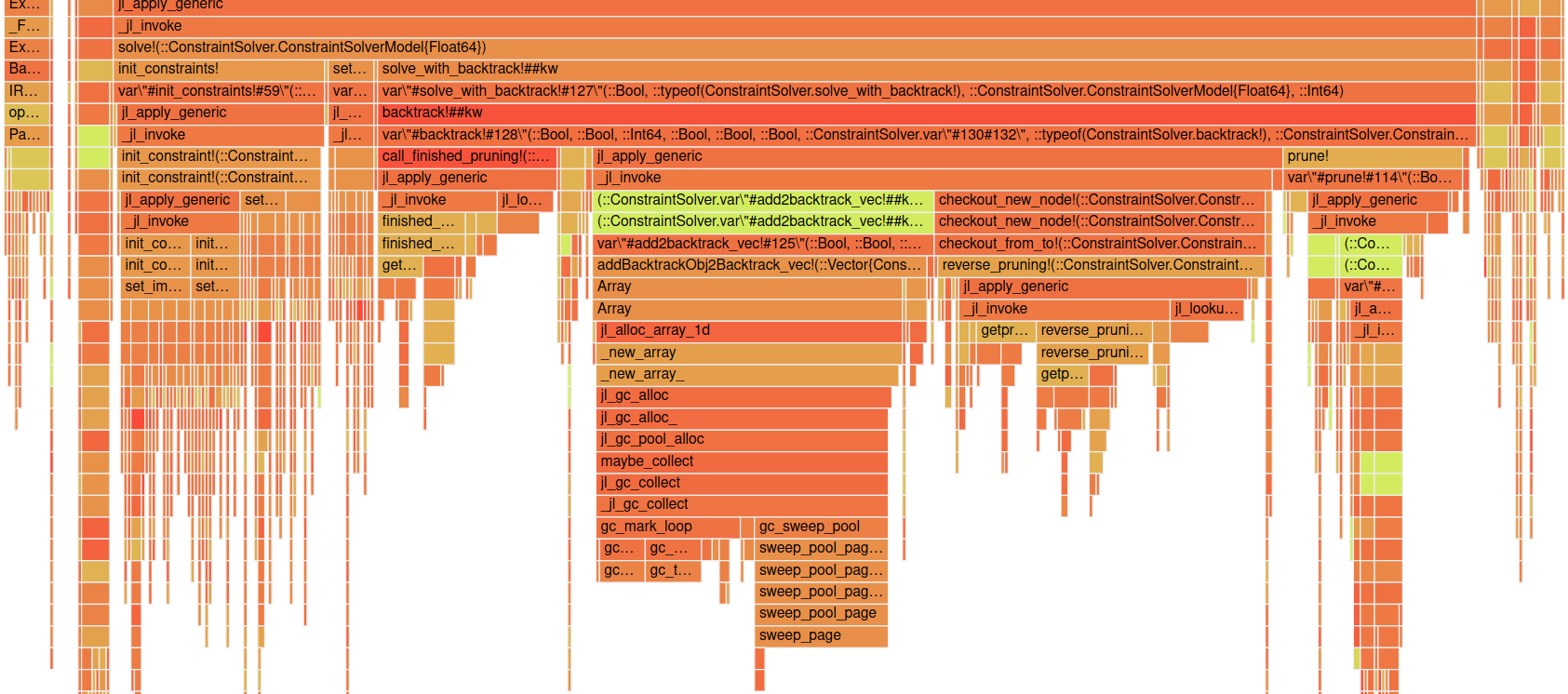
This can look a bit daunting at first but I think we understood how we can read it in general so let's step back a bit and just see which blocks are wide.
One thing you might see is this big Array block in the middle and _new_array below it. Seems like we are creating a lot of new arrays in between. This is something that we might be able to catch with track-allocation=user as well but this is a very quick way of getting a big overview.
The solver currently has about ~9K lines of code so just checking it line by line which might be a good approach for the prime function from before is not really feasible. In this post I don't want to have a look on how I resolved this issue but you might want to subscribe to the mail list to get notified about my next ConstraintSolver post 😉
Conclusion
Hope you've learned different ways to benchmark and profile your code using a variety of tools. There are some specific things that are not easy to see using these tools like type instability or bad memory layout but I felt these can often be avoided by having a basic understanding of those beforehand. I might do a blog post about these as well.
Additionally it's possible to have a look at a more lowered code level with some macros to dive deeper into some functions for micro optimizations which might be interesting for a future blog post as well.
List of other interesting tools and links you might want to have a look at
Performance Tips in Julia
ProfileView.jl similar to PProf but doesn't show it in a browser window but instead uses Gtk
Cthulhu finding type inference issues (I might use this in another post)
Thanks to my 11 patrons!
Special special thanks to my >4$ patrons. The ones I thought couldn't be found 😄
Site Wang
Gurvesh Sanghera
Szymon Bęczkowski
Colin Phillips
For a donation of a single dollar per month you get early access to these posts. Your support will increase the time I can spend on working on this blog.
There is also a special tier if you want to get some help for your own project. You can checkout my mentoring post if you're interested in that and feel free to write me an E-mail if you have questions: o.kroeger <at> opensourc.es
I'll keep you updated on Twitter OpenSourcES.
Want to be updated? Consider subscribing on Patreon for free
