B-splines
Creation date: 2019-08-24

About three month ago I published my post about Bézier curves and mentioned a follow up post about B-splines. Here it is ;) I finished the course on Geometric Modelling and Animation in university so I thought it's time now. Maybe there will be also a post on surfaces.
The blog post contains:
An explanation of B-splines
How to draw B-splines with different techniques
Normal way
De Boor Algorithm
Animations using Julia
What are B-splines?
The idea of splines in general is to combine several curves together to obtain one single curve. The curve itself should have some nice properties like continuity and it shouldn't behave in a strange way like making weird curves as a polynomial function of degree 15 might do. Another important point is local control which means if we move one control point a little bit we don't want to change the whole curve but only the small area around the point. For Bézier curves for example the whole curve can be changed even though the curve is changed mostly around the point that moved.
Additionally having a convex hull property is quite useful for collision detection as checking directly against the curve is quite complex which means it takes time whereas checking whether an object is inside a convex hull is easy. Later the tests can be refined if it at least has the possibility of being part of a collision with the actual curve.
In comparison to Bézier curves we gain local control, a better convex hull property and we can control the degree of the curve by combining curves together. Compared to Bézier splines we don't have to worry about A-frames anymore which was the last part of the previous post.
Let's have a look at a specific example:
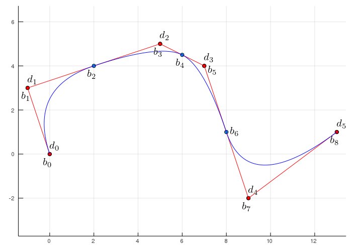
I have drawn this using my Bézier curve code of the last post and simple \(C^1\) continuity but for \(C^2\) this would be harder. In this example you can see the normal bezier points \(b_i\) and the so called de Boor points \(d_i\) which given the knot vector which I roughly explained last time (and the continuity) perfectly define the curve and the inner points \(b_2,b_4, b_6\) are defined implicitly by this.
I'll come back to the Knot vector later which defines the continuity and whether it is interpolating or approximating the point. For the comparison to Bézier splines it should be end point interpolating and approximating everywhere else which means that the curve touches \(d_0\) and \(d_{end}\) but not the ones in between.
I think we need a bit more definitions for the next steps:
We have \(m+1\) de Boor points, \(d_0,\dots,d_m\) which means in the example above \(m=5\) and degree \(n\) and the Knot Vector \(\mathbf{T} = (u_0, \dots, u_{n+m+1})\)
The spline is defined by:
\[ s(t) = \sum_{i=0}^{m} \mathbf{d}_iN_i^n(t) \]where \(N_i^n(t)\) are the B-spline basis functions which are defined by:
\[ N_i^0(t) = \begin{cases} 1 & \text{if } u_i \leq t < u_{i+1} \\ 0 & \text{else} \end{cases} \] \[ N_i^r(t) = \frac{t-u_i}{u_{i+r}-u_i}N_i^{r-1}(t) + \frac{u_{i+1+r}-t}{u_{i+1+r}-u_{i+1}} N_{i+1}^{r-1}(t) \quad 1 \leq r \leq n \]This can be easily implemented in Julia where we first define the basis function properties:
function b_spline_basis(i,r,t,u)
    u_i = u[i+1]
    u_i1 = u[i+2]
    u_ir = u[i+r+1]
    u_i1r = u[i+r+2]

    if r == 0
        if u_i <= t <= u_i1
            return 1
        else
            return 0
        end
    else
        N = b_spline_basis
        left = 0
        if (u_ir-u_i) != 0
            left = (t-u_i)/(u_ir-u_i) * N(i,r-1,t,u)
        end

        right = 0
        if (u_i1r-u_i1) != 0
            right = (u_i1r-t)/(u_i1r-u_i1) * N(i+1,r-1,t,u)
        end
        return left + right
    end
end
and then the plotting itself:
function b_spline(dBx,dBy, n, knot_vector; steps=200)
    m = length(dBx)-1
    if length(knot_vector) != m+1+n+1
        println("The knot vector has the wrong length it should have m+1+n+1 = ", m+1+n+1, " components.")
        println("But it has ", length(knot_vector), " components")
        return
    end
    plot(;size=(700,500), axisratio=:equal, legend=false)
    u_min = knot_vector[1]
    u_max = knot_vector[end]
    step_size = (u_max-u_min)/(steps-1)

    curve = zeros(steps,2)
    N = (i,r,t)->b_spline_basis(i,r,t,knot_vector)
    c = 1
    for t=u_min:step_size:u_max
        pos = zeros(2)
        for i=0:m
            if knot_vector[i+1] != knot_vector[i+1+n]
                pos = pos .+ [dBx[i+1],dBy[i+1]].*N(i,n,t)
            end
        end
        curve[c,:] .= pos
        c += 1
    end
    plot!(curve[:,1],curve[:,2])
    plot!(dBx,dBy, linetype=:scatter, color=:red)
    plot!(dBx,dBy, color=:red)
    for i in 0:length(dBx)-1
        annotate!(dBx[i+1]+0.2,dBy[i+1]+0.35, latexstring("d_"*string(i)))
    end

    png("b_spline")
end
then calling it using:
dBx = [0.0,-1,5,7, 9,13]
dBy = [0.0, 3,5,4,-2, 1]
@time b_spline(dBx, dBy, 2, [0,0,0,1,2,3,4,4,4])
I don't think that this is very elegant or fast and it's not reasonable to animate in this form.
The recursion depth is not very deep but recursion is not always the way to go. The de Boor algorithm is similar to the de Casteljau algorithm which I'll show you next. After that I'll show some examples of the knot vector to get a better understanding of what it means.
The de Boor Algorithm
We define a recursive scheme which we will implement similar to the de Casteljau algorithm using a loop. The scheme holds for \(u_l \leq t < u_{l+1}\):
\[ \mathbf{d}_i^0(t) = \mathbf{d}_i \quad \text{for } i=l-n,\dots,l \]and
\[ \mathbf{d}_i^r(t) = \Big(1-\frac{t-u_{i+r}}{u_{i+n+1}-u_{i+r}}\Big) \mathbf{d}_i^{r-1}(t) + \frac{t-u_{i+r}}{u_{i+n+1}-u_{i+r}} \mathbf{d}_{i+1}^{r-1}(t) \]for \(i=l-n, \dots,l-r\)
and the actual point is at \(\mathbf{d}_{l-n}^n(t)\) so we define a pyramidal scheme which uses the relevant de Boor points ranging from \(\mathbf{d}_{l-n}\) to \(\mathbf{d}_l\)
Now let's create some animations to get a better idea of the knot vector as you have seen above:
dBx = [0.0,-1,5,7, 9,13]
dBy = [0.0, 3,5,4,-2, 1]
b_spline(dBx, dBy, 2, [0,0,0,1,2,3,4,4,4])
I used a knot vector where the start and end knot is there three times (one more than the degree 2) and the rest is uniformly spaced.
In other words the start and end has a multiplicity of 3. Let's have a look what this means by changing the knot vector from [0,1,2,3,4,5,6,7,8] to [0,0,1,2,3,4,5,6,6] to [0,0,0,1,2,3,4,4,4].

As you can see there is no change in the curve between the first and the second one as the algorithm is the same (meaning the \(l\) evaluates to the same thing) but they are both not end point interpolating and therefore only the third is equivalent to a Bézier spline.
Before we test some property of the B-spline I want to change the knot vector in the middle by introducing a multiplicity there:
[0,0,0,1,2,3,4,5,5,5] to [0,0,0,1,1,2,4,5,5,5] to [0,0,0,1,1,1,4,5,5,5] to [0,0,0,1,1,1,1,5,5,5].
This changes the continuity of the curve for each multiplicity we reduce it by one.
(I added an extra point to have an even higher multiplicity)
As you can see for multiplicity 3 (degree + 1) we just connect the two de Boor points and for multiplicity 4 we skip one de Boor point.
The next thing I want to have a look at is to change one of the middle de Boor points to see whether that has an effect to the whole curve or not.
Here we can see that the curve only changes its shape in a small region of the entire curve.
The last thing I want to show is moving a point along the curve:
Thanks for reading!
I'll keep you updated if there are any news on this on Twitter OpenSourcES as well as my more personal one: Twitter Wikunia_de
If you enjoy the blog in general please consider a donation via Patreon. You can read my posts earlier than everyone else and keep this blog running.
Want to be updated? Consider subscribing on Patreon for free
