Bézier curves in Julia with animations

I think many heard about Bézier curves but maybe some of you didn't and I heard about it but wasn't really sure what they are and how they work. During my Geometric Modelling and Animations course in university we had some lectures on it and I did some coding for homeworks and also to understand a bit more about it. During the last days I published my animations on Twitter and asked whether you're interested in a post. There was quite a bit feedback on that so here it is!

Let us start with a basic Bézier curve:

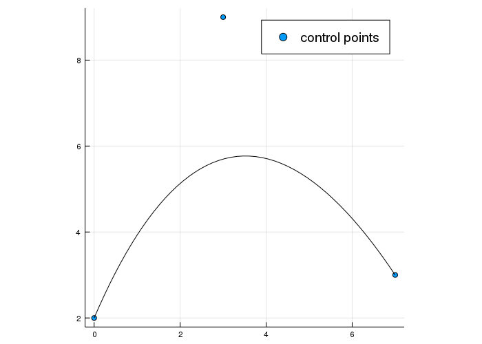
Before I show you what Bézier curves are we should probably have a short look what a basic curve is. A curve can be described by a parameterized description as:

\[ \mathbf{b}(t) = (x(t),y(t))^T \quad t_1 \leq t \leq t_2 \]

whereas \(\mathbf{b}\) is a vector and \(x, y\) are polynomial functions like

\[ x(t) = a_0 + a_1t + a_2t^2 + \dots + a_nt^n \]

Now the idea is to compute the values on the curve from \(t_1 = 0\) to \(t_2 = 1\) using a different basis not simply \(t^0, \dots, t^n\). For Bézier curves this basis are defined as:

\[ B_{i}^{n}(t) :=\left( \begin{array}{c}{n} \\ {i}\end{array}\right) t^{i}(1-t)^{n-i}, \quad 0 \leq i \leq n \]

and is called Bernstein basis.

Which looks a bit random for now but they have some interesting properties:

• \(B_{0}^{n}(t)+B_{1}^{n}(t)+\cdots+B_{n}^{n}(t)=1\)

• \(B_0^n(0) = 1, B_n^n(1)=1\)

which means when we write down the complete formula to compute \(\mathbf{b}(t)\):

\[ \mathbf{b}(t) = \sum_{i=0}^n B_i^n \mathbf{b}_i \]

where \(\mathbf{b}_i\) are our control points. Now the second property just means that \(\mathbf{b}(0) = \mathbf{b}_0\) and \(\mathbf{b}(1) = \mathbf{b}_n\)

I think it would be nice to actually see the basis functions.

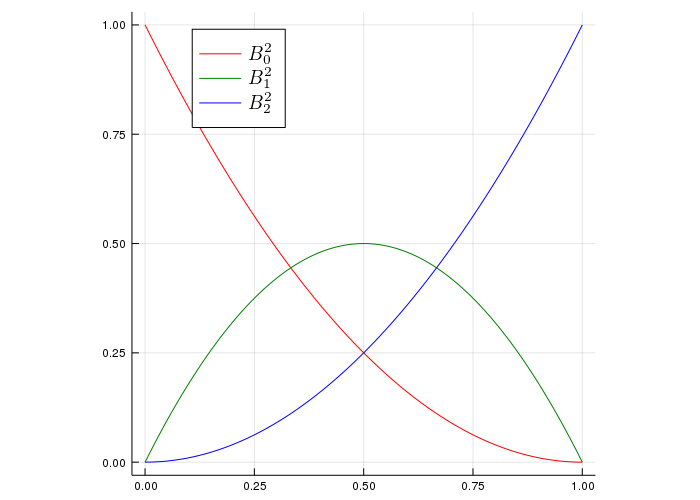
Here I used \(n=2\).

Now we can combine it with our control points to obtain:

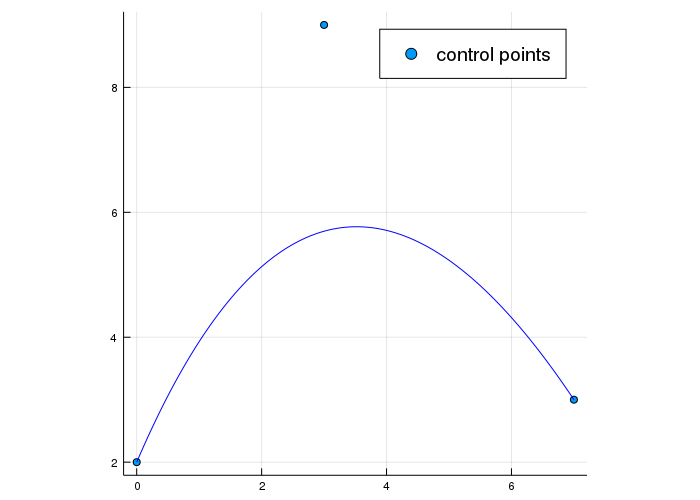
Besides the change in color you probably don't see a difference to the first plot even though that was plotted differently.

I know some of you are here for code so I'll show you the bernstein code:

using Plots
# for the LaTeX labels in the legend
using LaTeXStrings 

function compute_bernstein(i,n; steps=100)
    return [binomial(n,i)*t^i*(1-t)^(n-i) for t in LinRange(0,1,steps)]
end

function compute_bernstein_poly(px,py; steps=100)
    n = length(px)-1
    bernsteins = [compute_bernstein(i,n) for i=0:n]
    x_vals = [sum(px[k]*bernsteins[k][t] for k=1:n+1) for t=1:steps]
    y_vals = [sum(py[k]*bernsteins[k][t] for k=1:n+1) for t=1:steps]
    return x_vals, y_vals
end

function plot_with_bernstein(px,py; steps=100, subplot=1)
    x_vals, y_vals = compute_bernstein_poly(px,py; steps=steps)
    plot!(x_vals, y_vals, color=:blue, label="",subplot=subplot)
end

function main()
    px = [0, 3, 7]
    py = [2, 9, 3]

    plot(;size=(700,500), axisratio=:equal, legendfont=font(13))
    plot!(px, py, linetype=:scatter, label="control points")
    plot_with_bernstein(px,py)
    png("using_bernstein")
end

Pretty basic so far. Now combining the two and animate:

Actually I'm not too sure about how to interpret the colored animating part on the lower plot with the different bernstein polynomials but I think it looks interesting and I never saw that before. The three dots red, green and blue sum up to the black in both ways.

Anyway I think the interesting things are still missing. First of all we only have 3 control points at the moment maybe we want to increase that and on the other hand we have only one curve but it's possible to combine several curves and still have nice properties like \(C^2\) or \(G^2\) continuity. I'll give an explanation for the differences as well.

Bézier curves can also be computed in a recursive way which I actually did in the first plot but that can't be seen without animation.

\[ B_{i}^{n}(t)=(1-t) B_{i}^{n-1}(t)+t B_{i-1}^{n-1}(t) \]

So we compute the polynomial basis by itself by two lower order versions. The base cases are

\[ B_i^n(t) = 0 \text{ for } i < 0, i > n \text{ and } B_0^0(t) = 1 \]

This already looks like linear interpolation as we have \((1-t)\) and \(t\). The question is: Linear interpolation between which points?

Actually I think this is a nice transformation homework for you to do. From the recursion of Bernstein polynomials to the De Casteljau Algorithm which is stated like this:

\[ \begin{array}{l}{\mathbf{b}_{i}^{r}(t)=(1-t) \cdot \mathbf{b}_{i}^{r-1}(t)+t \cdot \mathbf{b}_{i+1}^{r-1}(t) \quad, \quad r \in\{1, \ldots, n\}, i \in\{0, \ldots, n-r\}} \\ {\mathbf{b}_{i}^{0}(t)=\mathbf{b}_{i}}\end{array} \]

Where \(b_i\) are our control points \(i \in \{0,..,n\}\) where n is the degree of the curve. In our examples it was always 2.

The points on the curve are \(b_0^n(t)\) with \(0 \leq t \leq 1\).

Now the change is basically that we have \(i\) and \(i+1\) instead of \(i\) and \(i-1\) and we included the control points directly into the formula.

I didn't implement it in a recursive fashion but instead building it up from the other side.

In our small example we have to compute \(b_0^2(t)\) which is based on \(b_0^1\) and \(b_1^1\) where which itself depend on \(b_2^0, b_1^0, b_0^0\) which are defined by the bézier points.

Let's have a look at our basic example in an animation:

For degree two we have three linear interpolations. From one bézier point to the next and then again from those two points. Always interpolating with \(t\) from the previous point and \(1-t\) weighted with the next point.

function animate_bezier(px,py;steps=100)
    n = length(px)-1
    # saving all in between de Casteljau points
    bs = [zeros(2,r) for r=n+1:-1:0]
    # base case Bézier points
    bs[1][1,:] = px 
    bs[1][2,:] = py
    points = zeros(steps,2)
    colors = [:green,:orange,:red,:yellow]
    c = 1
    anim = @animate for t in LinRange(0,1,steps)
        plot(;size=(700,500), axisratio=:equal, legend=false)
        plot!(px, py, linetype=:scatter)
        for i=1:n
            for j=0:n-i   
                # linear interpolation between twp ponts                   
                new_b = (1-t)*bs[i][:,j+1]+t*bs[i][:,j+2]
                bs[i+1][:,j+1] = new_b
                # drawing the line for linear interpolation as well as the specific point for t
                plot!(bs[i][1,j+1:j+2],bs[i][2,j+1:j+2], legend=false, color=colors[i])
                plot!([new_b[1]],[new_b[2]], linetype=:scatter, legend=false, color=colors[i])
                if i == n
                    points[c,:] = [new_b[1],new_b[2]]
                    # draw the curve until point t = LinRange(0,1,steps)[c]
                    plot!(points[1:c,1],points[1:c,2], color=:black)
                    c += 1
                end
            end
        end
    end
    gif(anim, "bezier_d2.gif", fps=30)
end

px,py are just the control/bézier points so we can add some and obtain this:

Before we come to the last part of this post (combining bezier curves) we can do something with this degree 4 Bézier curve which wasn't possible before. Actually there is more than one bezier curve.

Because of the recursive structure we can obtain curves of degree 3 as well now.

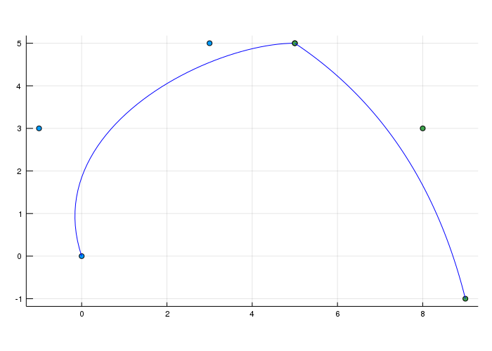
Okay the last part for today is about creating a curve which is the combination of two Bézier curves of degree three.

I think it's pretty clear that the end point of the first must be the starting point of the second to make it actually one curve.

It's quite obvious that this isn't what we want as everyone can clearly see that there is somehow a corner in the curve. Now there are possible restrictions we can have on the combination of two curves. The most basic one you can see above is the \(C^0\) and \(G^0\) continuity. The superscript basically tells us which degree of derivative is there the same. If you compute the tangent of the last point of the first curve and the tangent at the first point of the second curve they wouldn't be parallel/identical.

Actually it's quite easy to compute the derivative at the start and end point as well.

\[ \dot{\mathbf{b}}^{n}(0)=n\left(\mathbf{b}_{1}-\mathbf{b}_{0}\right), \quad \dot{\mathbf{b}}^{n}(1)=n\left(\mathbf{b}_{n}-\mathbf{b}_{n-1}\right) \]

I used these points:

px1 = [0.0,-1,3,5]
py1 = [0.0,3,5,5]

px2 = [5, 8, 9]
py2 = [5, 3, -1]

so for the left curve we need to compute \(n\left(\mathbf{b}_{n}-\mathbf{b}_{n-1}\right)\) where n = 3 so:

\[ 3\left(\mathbf{b}_{3}-\mathbf{b}_{2}\right) = 3 \begin{pmatrix} 5-3 \\ 5-5 \end{pmatrix} = \begin{pmatrix} 6 \\ 0 \end{pmatrix} \]

whereas for the second curve we obtain:

\[ n\left(\mathbf{b}_{1}-\mathbf{b}_{0}\right) = 3 \begin{pmatrix} 8-5 \\ 3-5 \end{pmatrix} = \begin{pmatrix} 9 \\ -6 \end{pmatrix} \]

This can be easily fixed by continuing on the line between the second last and last point of the first curve and place the second point of the second curve along that line. Then we have \(G^1\) continuity which means the tangents are parallel (well and they share the same end/start point) so they are \(C^0\) continuos as well. Now for \(C^1\) we want that the parametric representation of the curves has first derivative continuity. Which means that when we define the number of steps in the first curve as 200 for example and the number of steps 100 in the second curve but moving along the curve with 30 steps per second we spend more time on the first curve then on the second.

Now let's assume for a second that the point on the curve is travelling with constant speed on both curves (which isn't always the case and depends on the Bézier points) then at the merging point we would have an instant change in velocity which isn't always possible like if we are moving a camera along the curve.

In that case we want to have \(C^1\) or even \(C^2\) continuity which means there also isn't an instant change in acceleration. We get \(C^1\) simply by having the identical tangent (also the same length).

If we want to have \(C^2\) or \(G^2\) we can create a so called A-Frame:

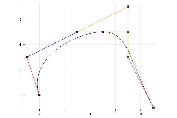
Here the following property must hold: The proportion between a orange and a parallel connected blue line must be \(\Delta_{i+1} : \Delta_i\). Now what is this \(\Delta_i\) ? It's \(u_{i+1} - u_i\) ah okay... Come on what is \(u\)??? Ah okay there is the problem. \(u_i\) is the ith component in the Knot vector \(\mathbf{U} = (u_0,u_i, \dots, u_L)\). Okay I swear this is the last part. The knot vector defines the time spend on a curve when the point arrives at \(u_i\). To make it simpler I decided to have an equidistant spaced Knot vector so that the blue lines are as long as the orange lines. (And yes the yellow line in the top left is orange :D)Somehow it's a problem that the line isn't flat and maybe has some aliasing issues or I don't know. Anyway back to the curves.

If we define the first curve with 4 points then we only have the choice of the last point of the second curve. The other three points are already defined by the \(C^2\) constraint.

For \(G^2\) on the other hand it's a bit more complicated but also we have a little more freedom and I'll not prove that the properties hold here. Just a graph to show how it can be constructed:

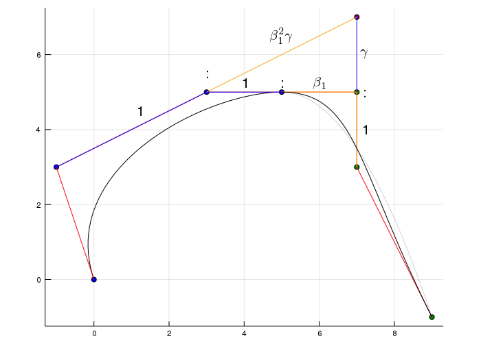
Now we have the freedom to choose \(\gamma\) and \(\beta_1\). Where

\[ \gamma=\frac{(n-1)\left(1+\beta_{1}\right)}{\beta_{2}+\beta_{1}(n-1)\left(1+\beta_{1}\right)} \]

can be defined by \(\beta_2\). For the last animation I used \(\beta_1 = 3\) and a range \(\beta_2\) from \(-30\) to \(30\).

I think you have all the necessary code components in this blog post. There are also other ways of computing and drawing bezier curves and the next topic would be b splines. If you enjoy this post and think it's reasonable to have a Julia Package or at least a repository for this code please make a comment. At the moment it's not that well organized so I decided not to publish my code in a repository this time. Anyway I think I open sourced enough so that everyone should be able to code this ;)

Update! I've created a new post in this short series that one is about B-splines. Check it out: Visual understanding of B-Splines

If you want to get more animations like this and earlier than everybody else => consider subscribing with Patreon to support this blog.

I'll keep you updated if there are any news on this on Twitter OpenSourcES as well as my more personal one: Twitter Wikunia_de

Thanks for reading!

If you enjoy the blog in general please consider a donation via Patreon. You can read my posts earlier than everyone else and keep this blog running.

Want to be updated? Consider subscribing on Patreon for free