Constraint Solver Part 4: Alldifferent constraint
Creation date: 2019-09-12

Series: Constraint Solver in Julia
This is part 4 of the series about: How to build a Constraint Programming solver?
Did you think about how humans solve sudokus?
At the moment we are simply removing values which are already set but what about a number which only exists once in possible values.
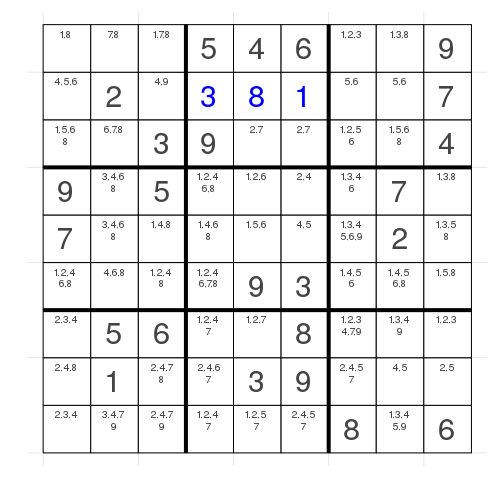
This is the example after the first post and in the penultimate row we have the following:
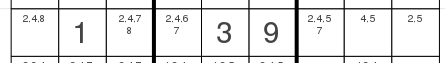
We clearly can set the value to 6 in the second block as we know that there has to be a six in the row (and also in the block) and it's the only choice for the six.
Let's have a look at another case in this grid. The second row is quite interesting as well:
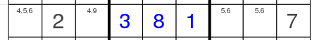
Here we have the possibilities 5 & 6 on the right block which means that we can't use 5 or 6 in the left part which fixes the left most value to 4 and the next to 9. We still don't know whether it's 5 and then 6 in the last block or 6 and 5 but we fixed two additional values.
Now the problem with the first part is a bit that maybe the 6 doesn't need to be fixed if we just want 9 values out of 10 or something (if we don't solve sudokus). We could check whether the number of values matches the number of indices.
The second one is not straightforward to implement I think and there a more thinks we could fix by doing some more reasoning.
In this post we will do some graph theory reasoning instead. Some of you might have read the post about Sudoku already but as this is a new series I want to explain it here again but will use the same visualizations as before.
I write about the implementation details in the end which are a bit messy at the moment in my opinion but not sure yet how to make it easier and being still fast or even faster so if you have some ideas ;) (actually writing it down in this blog made it less messy and faster :D)
Okay let's dive into graph theory: First of all want we want to do:
Create a graph where we connect our cells to the possible values we have in them.

The first row shows us the indices of the cells labeled a-i and the bottom row represents the values we have in general.
We might have some fixed values:

and then we add all the other edges which are possible:

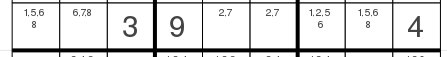
these are the possibilities of the third row in our sudoku:
I know the graph looks a bit full but we can add some color:

The green arrows show one possible matching. Now as mentioned several times in this series we always want to know as fast as possible if the current search space is infeasible or if we still believe that there might be a feasible solution.
It is clear that there is no feasible solution if there is no matching from indices to values such that every index is connected to one value and each value has at most (in sudoku: exactly one) corresponding index. The problem is known as finding the maximum matching in a bipartite graph.
A bipartite graph is a graph which has two blocks of nodes. A block of nodes here means that the nodes in this block are not connected to each other which is the case here: one block indices and one block values.
Now a maximum matching is a configuration where we want to mark the most edges (in our graph green) in such a way that the green edges don't share a start/end point.
You can get more information about Maximum Matchings on Wikipedia.
Okay so in this example we found a maximum matching of weight 9. The weight is normally the sum of all the weights of the edges and in our case all edges have weight 1.
Now we know it's feasible but we haven't removed any edges/possibilities yet.
If we could find all maximum matchings we could remove the edges which are not part of any of them.
Unfortunately it's not so easy to find all of them but fortunately there is a nice lemma about exactly what we need:
It says: An edge belongs to some but not all maximum matchings if and only if, given a maximum matching M, it belongs to either
an even alternating path starting at a free vertex
an even alternating cycle
A free vertex is a vertex which isn't part of the matching which we don't have in our sudoku problem. Attention: we have to care about it later for our general solver!
For now we concentrate on the even alternating cycles. An even alternating cycle is a cycle of even length and alternating means that we alternate between the green edges and the black edges.
This means we can make a directed graph and have the green edges in one direction and the black edges in the other such that all cycles we find are alternating as there is no way to choose a black edge after a black edge and it's even because we have a bipartite graph.
The directed graph looks like this:

Now let's have a look at a cycle:

Okay remove the green and black edges:

This means that those blue edges belong to some maximum matching and therefore can't be removed.
Now there are more cycles which you can all see here:


Now we have to remove all the edges which are green and or blue:

Let's have a look at the row in the Sudoku again to check whether that makes sense:
So the idea is now that we remove the value 2 from the 7th cell and the 7 from the 2nd cell. That makes sense!
Okay let's face the challenge of implementing it.
I use the MatrixNetworks.jl package which has functions for finding the maximum matching as well as the cycles.
To the coding part:
First of all we want to get the maximum matching where we can use the bipartite_matching function. It needs weights, the node indices in the first group and the node indices in the second group. So if a maps to 1,5 and 6 and b maps to 4 we would have the the weights [1,1,1,1] (weights are always 1) and then [1,1,1,2] for the second parameter and [1,5,6,4].
Reading it as:
[1,1,1,1]
[1,1,1,2]
[1,5,6,4]
So an edge is a column, with weights described by the first row, the second row is the one end of the edge and the third row the other end.
It's important that we use the numbers 1-9 each time even for our example where we have a sudoku with values 42,44,... as it internally would create all the other numbers in between starting from 1 which would use extra time and memory.
Therefore we need a mapping:
pval_mapping = zeros(Int, length(pvals))
vertex_mapping = Dict{Int,Int64}()
vertex_mapping_bw = Vector{Union{CartesianIndex,Int}}(undef, length(indices)+length(pvals))
vc = 1
for i in indices
    vertex_mapping_bw[vc] = i
    vc += 1
end
pvc = 1
for pv in pvals
    pval_mapping[pvc] = pv
    vertex_mapping[pv] = vc
    vertex_mapping_bw[vc] = pv
    vc += 1
    pvc += 1
end
num_nodes = vc
We have a mapping pval_mapping which maps an index from 1-number of pvals to the actual possible value. In the basic case of a sudoku it produces [1,2,3,4,5,6,7,8,9].
The vertex mapping maps a possible value to its vertex number so in our case 1-9 gets mapped to 10-18 as the first 1-9 are used by the indices and vertex_mapping_bw maps an index of the new graph to either a possible value or a CartesianIndex.
Then we want to count the number of edges we will have in the graph as we want to fill vectors of that size later as input for bipartite_matching instead of using push! as push! is slower.
# count the number of edges
num_edges = 0
@inbounds for i in indices
    if grid[i] != not_val
        num_edges += 1
    else
        if haskey(search_space,i)
            num_edges += length(keys(search_space[i]))
        end
    end
end
The @inbounds is a macro which we can use if we are sure that all the indices we use are valid then this gets a small speedup. It's not important here I think.
Now we can create two vectors ei which represents the second row of our small bipartite example above and ej the third row:
ei = Vector{Int64}(undef,num_edges)
ej = Vector{Int64}(undef,num_edges)

# add edge from each index to the possible values
edge_counter = 0
vc = 0
@inbounds for i in indices
    vc += 1
    if grid[i] != not_val
        edge_counter += 1
        ei[edge_counter] = vc
        ej[edge_counter] = vertex_mapping[grid[i]]-length(indices)
    else
        for pv in keys(search_space[i])
            edge_counter += 1
            ei[edge_counter] = vc
            ej[edge_counter] = vertex_mapping[pv]-length(indices)
        end
    end
end
Remember vertex_mapping translates a value to its vertex number which in our case would be 10-18 but we want low numbers starting from 1 so we subtract the number of indices.
Now we can get the bipartite matching:
# find maximum matching (weights are 1)
_weights = ones(Bool,num_edges)
maximum_matching = bipartite_matching(_weights,ei, ej)
if maximum_matching.weight != length(indices)
    logs && @warn "Infeasible (No maximum matching was found)"
    return ConstraintOutput(false, changed, pruned, fixed)
end
So if there is no maximum matching which includes every index we are sure that the problem is infeasible and can return.
Otherwise we have the maximum_matching object which has a field match which maps an index of the first block to the index of the second block.
So in our example
the output would be [1,6,3,9,2,7,5,8,4] which are the bottom indices of the green edges if we move from a to i.
Now we need the directed graph to get the cycles:
# directed edges for strongly connected components
di_ei = Vector{Int64}(undef,num_edges)
di_ej = Vector{Int64}(undef,num_edges)

vc = 0
edge_counter = 0
@inbounds for i in indices
    vc += 1
    if grid[i] != not_val
        edge_counter += 1
        di_ei[edge_counter] = vc
        di_ej[edge_counter] = vertex_mapping[grid[i]]
    else
        for pv in keys(search_space[i])
            edge_counter += 1
            if pv == pval_mapping[maximum_matching.match[vc]]
                di_ei[edge_counter] = vc
                di_ej[edge_counter] = vertex_mapping[pv]
            else
                di_ei[edge_counter] = vertex_mapping[pv]
                di_ej[edge_counter] = vc
            end
        end
    end
end
Here we will use the indices 1-18 as there is no assumption of being a bipartite graph anymore.
If a value is fixed we have a down arrow the same is true if the value is part of the maximum matching. Otherwise our arrow is going up.
Now for finding the cycles we can use sccs_map = strong_components_map(di_ei, di_ej) the function finds strongly connected components. A strongly connected component is a part of a graph where each vertex in that component can reach any other vertex in the component which is the case if there is a cycle.
As you can see above some vertices are in different cycles but a vertex is only part of a single strongly connected component. This means a strongly connected component might combine several cycles i.e if you have two cycles and they share one vertex then they are part of the same strongly connected component.
A vertex which is not part of a cycle has its own component of length one.
The sccs_map maps every vertex to its component id.
If two vertices are in the same component they are part of a cycle and therefore the edge between them is part of some maximum matching and therefore can't be removed.
Our last part is now to find all the edges which are not in the maximum matching and which endpoints are not in the same component as those edges are not part of any maximum matching and therefore can be removed:
# remove the left over edges from the search space
vmb = vertex_mapping_bw
for (src,dst) in zip(di_ei, di_ej)
    #  remove edges in same component
    if sccs_map[src] == sccs_map[dst]
        continue
    end
    #  remove edges in maximum matching
    if src <= length(indices) && dst == vertex_mapping[pval_mapping[maximum_matching.match[src]]]
        continue
    end

    cind = vmb[dst]
    delete!(search_space[cind], vmb[src])
    push!(pruned[cind], vmb[src])
    changed[cind] = true

    # if only one value possible make it fixed
    if length(search_space[cind]) == 1
        only_value = collect(keys(search_space[cind]))[1]
        feasible = fulfills_constraints(com, cind, only_value)
        if !feasible
            logs && @warn "The problem is infeasible"
            return ConstraintOutput(false, changed, pruned, fixed)
        end
        grid[cind] = only_value
        delete!(search_space, cind)
        push!(pruned[cind], grid[cind])
        changed[cind] = true
        fixed[cind] = true
    end
end
We iterate over each edge (zip helps to iterate over both end points at the same time)
If the endpoints have the same component id -> can't remove the edge.
If the edge is part of the maximum matching -> can't remove the edge
but otherwise we can remove the edge and therefore the corresponding value in one cell.
That's all we need. Now additionally we now work on the possible values and not only on the fixed values so we also want to fill the changed dictionary if we just make a change.
We will care about the problem of having more values than indices later in the series if you don't mind.
Hope you're excited about the benchmarks.
Benchmarks
As this is getting faster from time to time ;) and more people are reading I want to have better benchmarks. Instead of running it on my laptop where I sometimes have YouTube playing in the background or something I now run it on my workstation.
I have a 6 core Intel(R) Xeon(R) CPU E5-1650 0 @ 3.20GHz for comparison. I use version 1.1 of Julia.
Besides comparing it my solver to python-constraint and Norvig's solver...
Sorry I have to add that here: Do you know the birthday of Peter Norvig (Director of Research at Google)? The thing is the French and German Wikipedia mention the 12th of May and the English and Chinese version mention the 14th of December (actually the Chinese version also mentions the 4th of December in the text but the 14th of December in the Infobox.
Thanks for your help :D
... Okay I wanted to say I also compare it now to the shortest sudoku solvers I've ever seen: 43 lines of Python and compare it against the operations research tool by Google OR-Tools which is a general solver.
There are also some faster sudoku solvers but I think it's not reasonable to compare against those as I know that my solver will be much slower than something which is very specialized on this single goal.
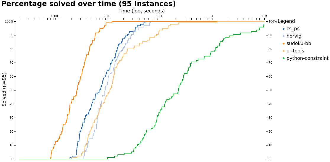
Our solver is the dark blue one. We are beating python-constraint by a factor of roughly 200 we also beat OR-tools and the sudoku solver by Peter Norvig but we currently have no chance against the specialized sudoku solver I found on GitHub.
For this post I have another two improvements and then will show you the benchmark performance again.
We always pass the CoM struct to all_different and that itself is not a huge problem but we didn't describe the type of our grid as best as possible. At the moment we have it declared as a AbstractArray but actually it is a Array{Int,2}.
Point 2 is that I had a look at the visualizations I made again and I saw quite often that it detects an infeasibility in the same cell in two different backtracking steps so thought why not use the cell next.
I mean having this get_weak_ind function now:
function get_weak_ind(com::CS.CoM)
    lowest_num_pvals = length(com.pvals)+1
    biggest_inf = -1
    best_ind = CartesianIndex(-1,-1)
    biggest_dependent = typemax(Int)
    found = false

    for ind in keys(com.grid)
        if com.grid[ind] == com.not_val
            num_pvals = length(com.search_space[ind])
            inf = com.bt_infeasible[ind]
            if inf >= biggest_inf
                if inf > biggest_inf || num_pvals < lowest_num_pvals
                    lowest_num_pvals = num_pvals
                    biggest_inf = inf
                    best_ind = ind
                    found = true
                end
            end
        end
    end
    return found, best_ind
end
And whenever we detect an infeasibility at a specific index we increase the bt_infeasible counter.

This brings us closer to the 43 lines of Python. I hate myself for being slower than 43 lines of Python :D
I hope you now believe that this can be a good constraint programming solver ;) Okay what's next? I am thinking about a different data structure but not too sure yet. Then we can do magic squares maybe.
Okay wait a second I have to do something about the tests. Don't worry it still passes the tests but the code coverage is very low because the new all different constraint is powerful so that no backtracking is needed.
So I add one sudoku from the hard test cases from the benchmark where some still need backtracking.
Further reading:
New post: Part 5: Different data structure
And as always:
Thanks for reading!
If you have any questions, comments or improvements on the way I code or write please comment here and or write me a mail o.kroeger@opensourc.es and for code feel free to open a PR on GitHub ConstraintSolver.jl
Additionally if you want to practice code reviews or something like that I would be more than happy to send you what I have before I publish. ;)
I'll keep you updated if there are any news on this on Twitter OpenSourcES as well as my more personal one: Twitter Wikunia_de
If you enjoy the blog in general please consider a donation via Patreon to keep this project running.
Want to be updated? Consider subscribing on Patreon for free
