Finding the maximum cardinality matching in a bipartite graph

Creation date: 2019-11-15

Tags: julia, constraint-programming, graph-theory

This is kind of part 14 of the series about: How to build a Constraint Programming solver? But it is also interesting for you if you don't care about constraint programming. In this post you'll learn about bipartite graphs and matchings.

Anyway these are the other posts so far in the ongoing series:

All of that can only happen because of the generous support of some people. I'm very happy that I can cover my server expenses now because of my Patrons. To keep this going please consider supporting this blog on Patreon. If you do I will create a better/faster blog experience soon and you will get posts like this earlier!

If you want to just keep reading -> Here you go ;)

Last time I realized that the library I'm using doesn't implement the easy algorithm I need which is bipartite maximum cardinality matching instead of bipartite maximum matching. This means they are solving a harder problem which I don't have :D

Additionally I like coding things from scratch so using a library is not the best choice but I am of course also limited in the amount of time I have and if people built it before it is often a good practice to not reinvent the wheel. Nevertheless this is a learning project where it is often good to know how a wheel works from the ground up.

The problem

We want to know whether a setting of numbers and possibilities in an all_different constraint is satisfiable or not.

For example we have 3 cells we want to fill with the numbers 1-3 and each should be used exactly once.

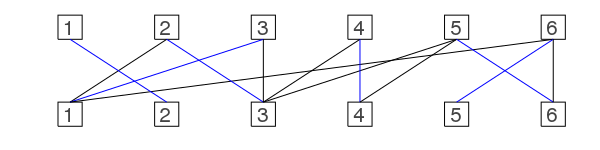
In the following examples our values are always at the top and the variables at the bottom. The goal is to match our variables to the values such that the all different constraint is satisfied. In this example there is no such matching:

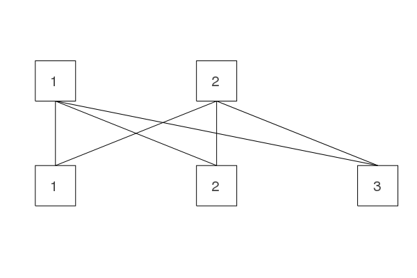
Bipartite maximum cardinality smaller than #values

In a more precise definition a matching is a set of edges such that two edges don't share the same vertex: Each vertex has at most one matching edge connected to it.

We are always interested in a matching which uses the most edges (maximum cardinality matching).

This is for example a matching (blue edges):

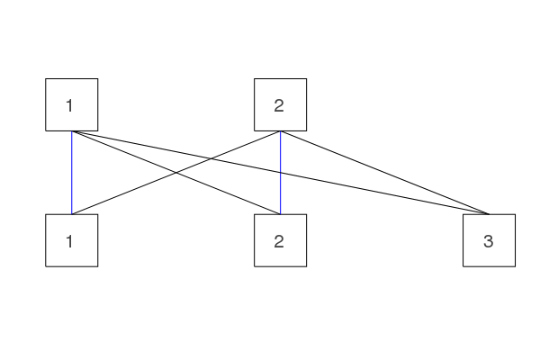
We need this maximum cardinality matching to check whether it is possible to fulfill the constraint and later to also remove edges which would make it impossible when used (explained in the all different section).

How can we find those matchings?

Let's have a look at a slightly bigger example:

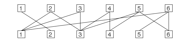
I should mention that these graphs are called bipartite graphs as they have two parts which are only connected to the other one but not to themselves. Yes there is a formal definition for it that you can look up :)

Now it's not that obvious anymore whether a matching with a cardinality of 6 exists.

Let's color in some edges which form a matching:

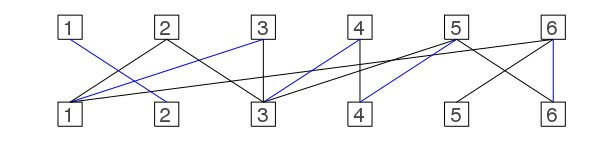
In the bottom row we have a so called unmatched vertex #5 (also called free vertex) and in the top row the 2 is unmatched. Which means there is no matching edge connected to it.

The matching can't be easily maximized as there is no edge from 5 to 2. (I say edges go up ;) )

The question remains whether there is a maximum cardinality matching with cardinality 6 as this one has only cardinality 5.

There is a quite simple idea to get a better matching if one exists:

We start at a free vertex, as my edges go up we start at a free vertex at the bottom, and if we find an alternating way to a free vertex at the top we can do something ;) An alternating way is a way that uses unmatched edges going up and matched edges going down. Actually we are looking for an augmenting path which is the name for an alternating path starting and ending at a free vertex and has an odd number of edges (starting at the bottom and end at the top).

green (up) / orange (down)

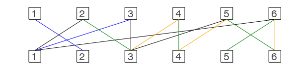
The nice thing now is that we can produce a new better matching by using the old blue edges + the green edges. The orange ones which were part of the matching before are now black.

It's quite simple and now we want to make it fast as our constraint solver should be as fast as possible ;)

Maybe some pseudo-code first:

Find initial matching
While bottom has free vertex
    Find augmenting path
    If not found 
        break
    Remove every second edge in the augmenting path from our matching
    Add every other edge of the augmenting path to our new matching

One can easily prove that this always increases our cardinality by 1 if there is such an augmenting path.

Before explaining my implementation I want to mention that <del>the same idea</del> a similar idea (see edit comment) can be used for general graphs not just bipartite once but I only need it for bipartite graphs and therefore the implementation is specialized to that for now.

Edit 18.11.2019: I'm very sorry for this mistake. I was questioned in my PR whether this works for general graphs with odd cycles. There is an algorithm for finding maximum matchings in general graphs: Blossom algorithm. Example where the algorithm you will read further down fails:

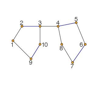
This is not important for the constraint solver as we only have bipartite graphs which don't have odd cycles but I had to correct my statement here.

We have 2 free vertices (2,8) and we can have an augmenting path: 1 -> 2 - 3 -> 4 - 5 -> 6 - 7 -> 8

But if we go 1 -> 9 - 10 -> 3 we can't find it and same is true if we start from 8 and go to 4 in the first step. Sorry for the wrong mention here before.

I'll make a PR to LightGraphsMatching.jl for the general case <del>soon</del> once I have understood the Blossom algorithm. Hope that doing some PRs there can help to revive that repository.

Implementation

Because I want to make the constraint solver faster I have some assumptions which might not hold for others. Besides the fact that the algorithm is for bipartite graphs I also assume that the first vector (in the examples this is the bottom part) has to be sorted (ascending).

This makes it easier to determine the neighbors of each bottom vertex.

The output of the function should be the same as for the bipartite_matching function in MatrixNetworks.jl. This means we want the matching output of the form of a vector with the same size as the number of vertices at the bottom. I call this length m and the length of the top n. Then an output like [1,4,5,2] would mean that the bottom vertex 1 (b1) is connected to the top vertex 1 (t1) as well as b2 - t2, b3 - t5, b4 - t2.

Important: For the constraint solver we only need to get a perfect matching if one exists or know that there is none. A perfect matching is a matching that uses every vertex. In our case only vertex at the bottom but don't know whether there is a different name for it. This is a bit easier than getting the maximum matching as we can return earlier if we know that there is no perfect matching without having to search for a better one than the current. Therefore I call the function bipartite_perfect_matching. Nevertheless it is very easy to change the functionality to find the maximum matching and is explained later on in the post.

function bipartite_perfect_matching(ei::Vector{Int}, ej::Vector{Int}, m, n)
    @assert length(ei) == length(ej)

    len = length(ei)
    matching_ei = zeros(Int, m)
    matching_ej = zeros(Int, n)

    # create initial matching
    match_len = 0
    for (ei_i,ej_i) in zip(ei,ej)
        if matching_ei[ei_i] == 0 && matching_ej[ej_i] == 0
            matching_ei[ei_i] = ej_i
            matching_ej[ej_i] = ei_i
            match_len += 1
        end
    end

    ...
end

matching_ei will be our main output later and besides having the structure mentioned above only for bottom to top I also have it the other way around.

The initial matching function basically iterates over the edges and tries to connect to connect free vertices if there is an edge. Which means for the most simple cases where we have a complete bipartite graph we can directly return a matching as it doesn't matter which maximum matching we take.

Now we have to check whether we found the maximum matching in the sense that we believe that there exists a matching as big as m or n. Maybe there isn't in which case our all_different constraint can not be satisfied.

The next step is to have a data structure which tells me in a fast way to which vertices a bottom vertex is connected to. Idea: Have a vector which tells you the first edge which corresponds to the bottom vertex this works as they are sorted by the bottom vertices.

Meaning: If I have ei: [1,1,1,1,2,2,2] I want to get [1,5,8] as the first index has edges from 1-4 the second from 5-7.

This can be done with where [1,5,8] is saved in index_ei.

# creating indices be able to get edges a vertex is connected to
# only works if l is sorted
index_ei = zeros(Int, m+1)
last = ei[1]
c = 2
@inbounds for i = 2:len
    if ei[i] != last
        index_ei[last+1] = c
        last = ei[i]
    end
    c += 1
end
index_ei[ei[end]+1] = c
index_ei[1] = 1

It's also possible to do that with cumsum:

cumsum(A; dims::Integer)                                                                                                                        
Cumulative sum along the dimension dims. See also cumsum! to use a preallocated output array, both for performance and to control the precision of  
the output (e.g. to avoid overflow).

For finding augmenting graphs we need to implement a breadth first search (BFS) algorithm. Therefore we need a list of nodes we want to process, depth information, who is the parent of a specific node in the BFS tree? And we need to keep track of all the nodes we visited already or more precise the ones we found already. For the last one I have two vectors one for the bottom nodes and one for the top ones.

A boolean variable indicates whether we found an augmenting path:

process_nodes = zeros(Int, m+n)
depths = zeros(Int, m+n)
parents = zeros(Int, m+n)
used_ei = zeros(Bool, m)
used_ej = zeros(Bool, n)
found = false

These stay the same if we have to find tenths of augmenting paths (we just overwrite them) this reduces the amount of memory allocation.

Then we have a loop for finding augmenting paths:

# find augmenting path
@inbounds while match_len < m
    pend = 1
    pstart = 1
    for ei_i in ei
        # free vertex
        if matching_ei[ei_i] == 0
            process_nodes[pstart] = ei_i
            depths[pstart] = 1
            break
        end
    end
    ...

Attention This only works if we are only interested in a perfect matching (a matching which uses every vertex). This is the case in our constraint solver. Otherwise one has to iterate over all free vertices until an augmenting path was found or all free vertices at the bottom have been checked. <- very important if you are interested in the general case

I missed that and only found it later as I am preparing a PR for LightGraphsMatching.jl. It's a small but important change which you can do by yourself or you can check out the PR at MatrixNetworks.jl

Here we find a free vertex and there exists at least one because we have match_len < m.

Then we have a loop over all process nodes which has the length pend and the current pointer of the start as pstart. Therefore while pstart <= pend means as long as the process nodes has a node which we didn't process yet.

while pstart <= pend
    node = process_nodes[pstart]
    depth = depths[pstart]

    # from bottom to top
    if depth % 2 == 1
        # only works if ei is sorted
        for ej_i = index_ei[node]:index_ei[node+1]-1
            child_node = ej[ej_i]
            # don't use matching edge
            if matching_ej[child_node] != node && !used_ej[child_node]
                used_ej[child_node] = true
                pend += 1
                depths[pend] = depth+1
                process_nodes[pend] = child_node
                parents[pend] = pstart
            end
        end
    else ...

as we are in a bipartite graph we know based on the depth whether we are currently at the bottom or at the top. The function above is for the nodes from bottom to top. We have the indexing vector index_ei to iterate over the neighboring top nodes. At this stage we want to use edges which are not part of the matching and because we in general don't want to visit nodes we already visited. If we found one of those edges we set the connected node as visited and add it to depth, process_nodes and parents.

In the else statement this is ej -> ei or here top to bottom. Here we only want matching edges because this is how augmenting paths are defined.

else 
# if matching edge
match_to = matching_ej[node]
if match_to != 0
    if !used_ei[match_to]
        used_ei[match_to] = true
        pend += 1
        depths[pend] = depth+1
        process_nodes[pend] = match_to
        parents[pend] = pstart
    end
else ...

If match_to != 0 it means we have a matching edge so we want to just traverse it similar as before. Otherwise we found an augmenting path then we basically want to go the steps back and remove the edges from the matching we visited on the path and were matching edges and adding the other augmenting path edges to the matching.

# found augmenting path
parent = pstart
last = 0
c = 0
while parent != 0
    current = process_nodes[parent]
    if last != 0 
        if c % 2 == 1
            matching_ej[last] = current
            matching_ei[current] = last
        end
    end
    c += 1
    last = current
    parent = parents[parent]
end
# break because we found a path
found = true
break

Here I basically don't remove edges from the matching as I can just overwrite them.

After closing some if and else we continue with the next process node so pstart += 1.

Then there are two options either we found an augmenting path in the while loop or there is none.

if found
    match_len += 1
    if match_len < m
        used_ei .= false
        used_ej .= false
    end
    found = false
else 
    break
end

At the end of the function we have:

return Matching_output(m, n, match_len, match_len, matching_ei)

MatrixNetworks uses:

mutable struct Matching_output
    m::Int64
    n::Int64
    weight::Float64
    cardinality::Int64
    match::Array{Int64,1}
end

I've added this to the ConstraintSolver as well as made a PR. There I implemented the actual algorithm which I described in the Attention part above.

There are better algorithms for this like the Hopcroft Karp algorithm which basically does the same but takes several augmenting paths at once. I think it's not necessary for small all_different constraints which is the reason why I dropped it for now but might come back to it.

Benchmarks

I did a benchmarking update about three weeks ago and since then there was the memory post and this one so let's have a look at the new version. I didn't change graph coloring so that stays the same.

Short mention on these benchmarks: I know and you should too that it's a bad idea in general to use my solver instead of the sophisticated OR-Tools. I do these benchmarks to have some kind of comparison. My solver can solve only very view kinds of problems at the moment compared to OR-Tools. These benchmarks should just give an overview and shell show the improvement during this process of creating the constraint solver. If I see that OR-Tools is much faster I know that there is some kind of improvement and I can look for it but without it I can only get: Ah okay my solver takes 2 seconds... Is that any good? If you're interested in how to do unbiased benchmarks please read Biased benchmarks by Matthew Rocklin To be clear I don't assume the following to be unbiased in any way :)

Killer sudokus:

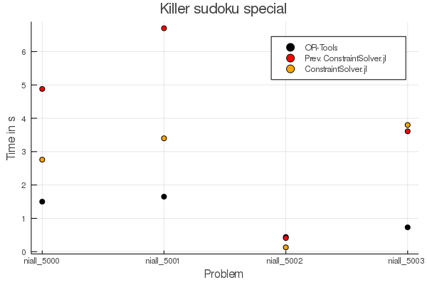
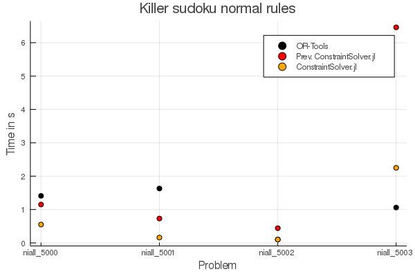
You can see that in some cases there is a drastic improvement and only for one case it takes a bit longer than before. For Killer sudokus with normal rules we are faster in three of four cases and slower in one case. (For niall_5002) OR-Tools takes the same time as the new Constraint Solver version :)

Let's have a look at the sudoku case:

We are now as fast as the sudoku-bb solver.

One thing that can be improved now that I wrote the matching algorithm is that we can reuse the memory so each all_different constraint can get the memory for process_nodes , depth and so on once and just reuse it. (See issue #49).

A new post is out: Making the solver a JuMP solver!

Some more things:

Kaggle challenge

As of now the Kaggle challenge Santa 2019 didn't start yet. Once it does I'll have a look at it and blog about it as soon as possible. Explaining the problem first and some ideas probably and work on it the next weeks then and keep you posted as this time I'll not go for winning a medal but instead gaining some followers for the blog from the Kaggle community ;)

What's next?

There are some things missing:

Hopcroft Karp bipartite matching
reuse memory in bipartite matching
Trying to speed up the sum constraint
- Only one bit takes a bit memory which maybe can be reduced
Looking at the search tree for bigger graph coloring

Stay tuned ;)

And as always:

Thanks for reading and special thanks to my four patrons!

List of patrons paying more than 2$ per month:

Site Wang
Gurvesh Sanghera

Currently I get 9$ per Month using Patreon and PayPal when I reach my next goal of 50$ per month I'll create a faster blog which will also have a better layout:

Code which I refer to on the side
Code diffs for changes
Easier navigation with Series like Simplex and Constraint Programming
- instead of having X constraint programming posts on the home page
And more

If you have ideas => Please contact me!

If you want to support me and this blog please consider a donation via Patreon or via GitHub to keep this project running.

For a donation of a single dollar per month you get early access to the posts. Try it out for the last two weeks of October for free and if you don't enjoy it just cancel your subscription.

If you have any questions, comments or improvements on the way I code or write please comment here and or write me a mail o.kroeger@opensourc.es and for code feel free to open a PR on GitHub ConstraintSolver.jl

I'll keep you updated on Twitter OpenSourcES as well as my more personal one: Twitter Wikunia_de

Want to be updated? Consider subscribing and receiving a mail whenever a new post comes out.

Subscribe to RSS

OpenSourc.ES