Graph Coloring using Cliques

Welcome back everyone to a new post on the development of the ConstraintSolver Julia package.

If you have missed previous posts on the development you might want to start at the beginning of this long series. Start of the endeavour of building a constraint solver in Julia. You can also have a look at all posts in the topic by topic list when you open the menu on the top left.

This post basically builds on top of the graph coloring post and graph coloring compared to MIP. Nevertheless I'll shortly explain what we did before here as it's more than a year ago...

Very short introduction into the ConstraintSolver.jl package

I've started in September 2019 to build a constraint solver almost from scratch. One can say it all started with trying to solve sudokus like humans do and escalated quickly. A constraint solver basically takes in a number of variables, constraints and sometimes an objective function. Then tries to optimize the objective function and fulfilling all the given constraints.

In comparison to linear programming or mixed integer programming the current variant only accepts integer variables. The biggest difference is that constraints don't really have to obey any rules. For linear programming they have to be linear which makes sense.

The constraint solver currently accepts the same constraints plus:

• AllDifferent

  • Which can be used to solve sudokus with the constraint that all digits in a row, column and box have to be different from each other

• TableConstraint

  • One can specify a list of possible values for a set of variables as a table. The tables might get huge but you basically have a way to define whatever you want by simply enumerating all possibilities. (Should only be used if there aren't trillions of combinations 😄)

• IndicatorConstraint

  • Something like: b => {x+y+1 == 5} such that the constraint only holds if b is 1 (here b is always binary).

• ReifiedConstraint

  • Kind of the opposite of IndicatorConstraint: b := {x+y+1 == 5} means b is 1 if the constraint is fulfilled.

• !=

  • Linear programming allows: a + b <= c and a + b == c but not a + b != c. The constraint solver does.

More constraints can be added and will be added in the future.

I think one can see the benefits of a constraint solver. It has of course downsides when one actually wants to solve an integer linear program as it isn't as specialized.

How it works

Well you might want to start at the beginning but in general it works like this:

Every constraint can prune the search space and can check whether the constraint is still fulfilled if one sets a value.

As an example let say we have a = 0:5, b = 0:5 and c = -5:5

For a + b == c we can reduce the search space of c to 0:5 as negative numbers can't be reached.

If a,b and c should be all different we can't do anything at the moment but if we set a = 0 during our search we can remove the value from b and c. Often we can do much more than these simple != operations. More on that in the first few posts and it's also the idea for later.

We apply those pruning steps as long as we can prune something and then we test out a value, prune again and backtrack if it doesn't work.

Alright that should be it for the basics 😉

How we currently solve graph coloring problems

Let's have a look at how we currently color a graph and explain the problem in general.

We have a graph with ten vertices (\(|V|=10\)) and a bunch of edges \(|E|=18\).

Our goal is to find a coloring of the vertices such that two connected vertices (one calls them adjacent) don't have the same color.

In previous posts we saw that one can use this to color maps in a way that two neighboring states/countries are distinguishable.

Nevertheless graph coloring is more complicated than that as there is an upper bound for the number of colors needed for maps (see The Four Color Map Theorem - Numberphile)

Generally we are looking for using the minimum amount of colors otherwise you could trivially use \(|V|\) colors.

The naive implementation from a year ago simply used the != constraint for each edge i.e

using ConstraintSolver, JuMP
const CS = ConstraintSolver

n = 10
m = Model(CS.Optimizer)
@variable(m, 1 <= c[1:n] <= n, Int)
@variable(m, 1 <= max_color <= n, Int)

edge_list = [(1,2), (1,5), (1,7), (1,8),
            (2,4), (2,7), (2,8), (2,9),
            (3,7), (3,9), (3,10),
            (4,9), (4,10),
            (5,10),
            (6,7), (6,9),
            (7,8), (7,10)];

for edge in edge_list
    @constraint(m, c[edge[1]] != c[edge[2]])
end

@constraint(m, max_color .>= c)
@objective(m, Min, max_color)

optimize!(m)
status = JuMP.termination_status(m)
objval = JuMP.objective_value(m)
solve_time = JuMP.solve_time(m)

println("Status: $status")
println("Number of colors needed: $objval")
println("Time for solving: $solve_time")

which prints out:

# Variables: 11
# Constraints: 28
 - # Inequality: 10
 - # Notequal: 18

   #Open      #Closed         Incumbent     Best Bound        Time [s]  
========================================================================
     1           1                -            2.00            0.0003   
     11          27              4.00          4.00            0.001 

Status: OPTIMAL
Number of colors needed: 4.0
Time for solving: 0.0012619495391845703

I thought I just show you the code as it's quite short.

It shows that we need four colors so my coloring from before, which I did by hand, is optimal 😉

That version basically tries out a color and removes it from its neighbors and if one node doesn't get a color it means we failed and have to backtrack. Normally backtracking doesn't happen that often as it's hard to fail when we allow \(|V|\) colors. It's more that we try out a different node in our search tree if it has a better bound.

Idea for improvements

Above you can see the results which we currently have. There it struck me that the first best bound is 2.0. Which is very low but it makes sense as that is all we know with a != constraint.

How can we improve that lower bound?

Let's have a look at the graph again:

The vertices 1, 2 and 8 are forming a triangle. This already means that the lower bound is to use three colors as those three vertices need to have all different colors.

If we look more closely we can actually see that they are also all connected to the 7. This implies we have a lower bound of 4.

When we know that we don't need to search for a solution with 3 nodes and try out another node. We can directly look for a solution with four nodes.

In more technical terms we are looking for cliques in the graph. A clique is a set of nodes which are all connected to each other.

Actually to be more precise we are looking for the maximum clique in the graph to get the lower bound. What we later do is to actually search for all maximal cliques.

A clique is maximal if we can't add another node to it to make it bigger i.e 1,2 and 8 form a clique but only with the 7 it's a maximal clique.

Two connected nodes also form a clique btw, but it's not really interesting.

Let's have a look at all maximal cliques of size 3 and 4 in this graph.

How to implement this?

The question is how to apply that knowledge to the problem.

If we think a bit more about this we might realize that the cliques form an all different constraint.

We can therefore remove some != constraints and combine them to all different constraints.

I think this is nothing we expect from the user to do so we internally have to combine them. The constraint solver has a simplify method for things like that which can add constraints. With this implementation we also want to be able to delete constraints.

Let's have a high level overview of what needs to be done as I honestly don't wanna show much code here. You can check out PR 188.

I've came across the maximal_cliques function in LightGraphs.jl. Therefore, we only need to create the graph, call the function and combine the nodes that are part of a clique into an all different constraint.

This is already helpful but doesn't actually set the bound because we somehow need to compute the bound. At this stage the solver simply knows we want to minimize a single variable and that the max_color variable is bigger or equal to the rest of the variables.

In each step where we set a color we can prune the minimum number of our max color variable, but we don't start with something initially which is better than before.

We need to combine all the max_color >= vertex_color constraints into a single constraint which combines the power. There we can check whether there are any all different constraints completely covered by our new vector constraint.

Okay I might be moving a bit fast here.

What I mean is we create a constraint [max_color, x...] in GeqSet() which means the same as the \(|V|\) >= constraints we had before but are part of a single constraint. (We can do this in simplify as well).

Then we check if there is an all different constraint which variables are completely covered by the second part of the GeqSet constraint. If that is the case we can extract information. If we have [1:5, 1:5, 1:5, 1:5] as a part of x and it's part of an all different constraint we can obtain the minimum as a permutation of [1,2,3,4] so we need at least the value 4. This can be set as our upper bound.

The last thing we want to do is to use the power of a linear programming solver to get us the best bound from all the variable bounds we have. This isn't strictly necessary here but makes it easier to implement for us.

One needs to replace m = Model(CS.Optimizer) with:

using Cbc
cbc_optimizer = optimizer_with_attributes(Cbc.Optimizer, "logLevel" => 0)
m = Model(
    optimizer_with_attributes(
        CS.Optimizer, 
        "logging" => [], "lp_optimizer" => cbc_optimizer
    )
)

to use this power. Then every constraint is able to add an extra variable to the linear program (LP) and sets its bounds.

Example

Before we have a look at the benchmarks let us have a look at our example from above and how it gets colored.

• We start with coloring the vertex 1 with green.

  • This removes the color from all neighbors (2,5,7,8)

• In the next step we choose the vertex 2 and color it blue

  • This restricts (7,8) even further and also restricts 4 and 9.

• and so on until all vertices have colors

Benchmarks

We always want to make sure that we actually improve the running time, right? Therefore we need to find benchmark sets and test our previous version with the new.

In this case I found Graph Coloring Benchmarks which lists some instances in certain categories. I had a look at the ones which can be solved in less than a minute by using a state-of-the-art solver.

You can see in a second that I'm not one of them 😉

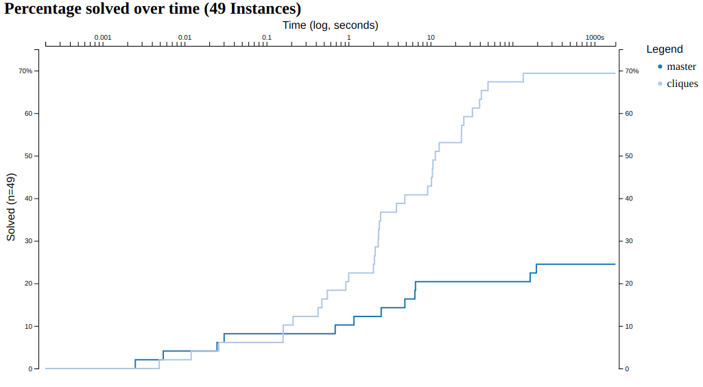
I've downloaded 49 instances and compared my two implementations. One can see that a bit less than 70% of the instances can be solved in less than 3 minutes with our clique implementation.

Whereas, with the current master version of the constraint solver only 20% of the instances can be solved that fast. My time limit was 30 minutes and there is unfortunately no improvement after about three minutes for the new version. The current version of ConstraintSolver can solve a few instances more with extra time but can barely solve a quarter of the "easy" instances in half an hour.

Further improvements

One can clearly see that we are not done yet but we made some good progress.

My goal is to solve 100% in less than 5 minutes in general but first of all do it in less than half an hour 😉

Let's talk about some problems and possible further improvements.

It's an NP-hard problem to find all maximal cliques such that for one of the 49 instances the solver didn't even start the search procedure in the time limit. Maybe it's possible to find maximal cliques with an heuristic as it isn't super important that I find all of them.

I'm sure there are some more smart ways to speed this up. There might be some ways for finding a solution faster with a better search strategy like activity based search which I currently try in a different branch.

Anyway this is now part of the new release v0.4. Feel free to check it out: ConstraintSolver .

Thanks everyone for checking out my blog!

Special thanks to my 10 patrons!

Special special thanks to my >4$ patrons. The ones I thought couldn't be found 😄

• Site Wang

• Gurvesh Sanghera

• Szymon Bęczkowski

• DShiu

For a donation of a single dollar per month you get early access to these posts. Your support will increase the time I can spend on working on this blog.

There is also a special tier if you want to get some help for your own project. You can checkout my mentoring post if you're interested in that and feel free to write me an E-mail if you have questions: o.kroeger <at> opensourc.es

I'll keep you updated on Twitter OpenSourcES.

Want to be updated? Consider subscribing and receiving a mail whenever a new post comes out.

Enter your email

Powered by Buttondown.