Constraint Solver Part 11: Graph Coloring Part 2
Creation date: 2019-10-18

Series: Constraint Solver in Julia
This is part 11 of the series about: How to build a Constraint Programming solver?
In the last post we created the != constraint to solve graph coloring. The problem is that we currently can't specify that we want to minimize the number of colors used. We therefore tried it out with four colors because based on the four color theorem this should work and well it did. After that we checked whether that is the best solution by removing the fourth color. It turned out to be infeasible.
I want to add the possibility to optimize in this post. We have to keep track of a bit more information for this which we will do first before implementing the optimization step.
First of all I want to show you another interesting way to solve graph coloring using Mixed Integer Programming (MIP). I did a series on how to solve linear problems (see Simplex Method) and also a post on how to use a MIP solver to solve small Travelling Salesman Problems TSP solver.
Comparison with MIP
Let's compare our current constraint solver approach without optimization step with a MIP approach. We will use GLPK.jl which is a wrapper to call GLPK in Julia. It works using JuMP.jl which is the Julia package for mathematical programming.
I got the idea from this blog post on graph coloring written in R.
What are the rules? Or how can we write the graph coloring problem as a mixed integer (here actually all variables are integer) linear problem?
We could use the same variable structure:
A variable for each state having the possible values 1,2,3 & 4
but it's not that easy to have a != in a linear problem. Therefore we use a different approach namely we have four binary variables for each state. If we don't know the four color theorem we need to add more colors same is true if we don't actually have a valid 2D Map. Graph coloring can also be used if we have a graph of nodes and edges we want to separate the nodes in such a way that two connected nodes don't have the same color.
Pseudocode:
c[s][1,2,3,4] = {0,1}c[1][1] = 1 would mean that we use color 1 (red) for the state of Washington which was the first in our list of states.
The first constraint then is quite obvious
\[ \sum_{i=1}^4 c[s][i] = 1 \quad \forall s \in \text{States} \]Meaning: Each state has exactly one color.
Now we also want to minimize the number of colors we use. It's the easiest to introduce a new variable max_color for this.
Objective:
\[ \min \text{max\_color} \]How is max_color connected with the actual maximum color?
Which means max_color has to be bigger or equal to the product of the value of the color 1,2,3 or 4 with the variable which indicates whether this color was actually chosen.
You might wonder: Okay but it can be way higher, right? Like 20. Yes we don't restrict it from above but it gets minimized by our objective so in the end it will be the actual maximum color.
If we would implement just these rules the result would be that c[s][1] = 1 for every state to make max_color = 1. We of course have to add the constraint that neighboring states are not allowed to have the same color.
Basically:
\[ c[s][i] + c[n][i] \leq 1 \quad \forall s \in \text{States}, n \in \text{neighbors of s} \]That means they can't both have a 1 but both might have a 0 of course.
Now I don't want two identical constraints as all neighbors of s also have s as a neighbor. We can limit this by saying \(n > s\).
I hard coded all the constraints in the first post so I'll just use that.
This is outside the constraint solver so you can download the code here: Gist Link
If you don't have JuMP.jl and GLPK.jl installed you need to run:
] add JuMP
] add GLPK
In JuMP it looks like this:
using JuMP, GLPK

m = Model(with_optimizer(GLPK.Optimizer))

@variable(m, max_color, Int)
@variable(m, c[1:49,1:4], Bin)

@objective(m, Min, max_color)

for s=1:49
    @constraint(m, sum(c[s,1:4]) == 1)
end

for s=1:49, i=1:4
    @constraint(m, max_color >= i*c[s,i])
end

for i=1:4
    @constraint(m, c[1,i] + c[11,i] <= 1)
    @constraint(m, c[1,i] + c[8,i] <= 1)
    ...
end

optimize!(m)
println(JuMP.objective_value(m))
println(JuMP.termination_status(m))
You can access the color variables using JuMP.value(c[1,1]) to check whether we set Washington to red or to get the color we set Washington to:
_, color_washington = findmax(JuMP.value.(c[1,:]))
println("color_washington: ", color_washington)
or you can write it more elegantly if you define the neighbors of each state first.
The m = Model line specifies which solver we want to use. There are commercial solvers like Gurobi which will be much faster for bigger problems than GLPK which we are using now. You might also want to check out Cbc.jl which you could use with:
using Cbc
m = Model(with_optimizer(Cbc.Optimizer, logLevel=0))
If we benchmark this using GLPK it takes about 0.2 seconds on my machine which is quite slow I think. We could continue with the constraint solver now and just leave it like that having a slow baseline algorithm. But of course we don't do that!
How does a MIP solver approaches the problem?
It solves the so called relaxation first that means it ignores the discrete constraint on the color variables. If you are the computer and you're very lazy what would you like to do?
Setting the objective to the lowest value possible
We have these constraints:
for s=1:49, i=1:4
    @constraint(m, max_color >= i*c[s,i])
end
And c is binary which means in the relaxed form it is between 0 and 1 \(\implies \text{max\_color} \geq 0\).
But the sum of all colors for each state has to equal 1 and we have the neighbor constraints.
What we can do is set everything to \(0.25\) then we have max_color = 1, the sum is \(4*0.25=1\) and all the neighbor constraints add up to \(0.25+0.25=0.5\).
Ah damn we assumed again that max_color is discrete... We have to be more evil. We can actually set the variables for each country to. [0.48, 0.24, 0.16, 0.12] This sets max_color to be equal to 0.48.
Every constraint is fulfilled but we have no information at all. Now we would pick one of those variables and create a tree like structure.
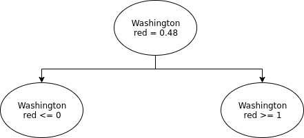
We would create two sub problems one where we fix Washington red to 0 and one were we fix it to 1. The solver would now choose the one were it is set to 0 maybe as it still believes that we can color everything with max_color=1. And set the other three options of Washington to something evil which only marginally increases the max_color.
How can we solve this problem?
Ideally we would like to have if we use a bit of the second color this should immediately set the max_color to 2 but that's not doable. What we can do is that instead of
for s=1:49, i=1:4
    @constraint(m, max_color >= i*c[s,i])
end
we use the sum over all colors of a state multiply it by the number of the color (1...4) and set max_color has to be bigger or equal to that.
In the [0.48, 0.24, 0.16, 0.12] case we had before this would add up to \(1.92\) instead of \(0.48\) and it reduces the number of constraints which might also be helpful. In our US coloring case it finds a way to set the variables in such a way that max_color = 1.5 but it's better than 0.48.
Now it only takes 0.04 seconds.
Lesson learned: With MIP try to have a look at an evil MIP solver which tries to find the best solution without discrete values. Then try to reformulate the constraints such that this isn't beneficial anymore for the evil solver.
If you want to get more information from the solver in those cases you can use m = Model(with_optimizer(GLPK.Optimizer, msg_lev = 3)) for GLPK and every other solver has also some kind of logging option.
GLPK Simplex Optimizer, v4.64
669 rows, 197 columns, 1436 non-zeros
      0: obj =   0.000000000e+00 inf =   4.900e+01 (49)
    167: obj =   6.666666667e-01 inf =   7.772e-16 (0)
*   231: obj =   4.800000000e-01 inf =   3.775e-15 (0)
OPTIMAL LP SOLUTION FOUND
GLPK Integer Optimizer, v4.64
669 rows, 197 columns, 1436 non-zeros
197 integer variables, 196 of which are binary
Integer optimization begins...
+   231: mip =     not found yet >=              -inf        (1; 0)
+   698: >>>>>   4.000000000e+00 >=   3.000000000e+00  25.0% (66; 2)
+  5008: mip =   4.000000000e+00 >=     tree is empty   0.0% (0; 273)
INTEGER OPTIMAL SOLUTION FOUND
The number of rows columns and non-zeros might be interesting.
Rows: number of constraints
Columns: number of variables
Non-zeros: Number of non zeros in the simplex matrix. Maybe check out Simplex Method in Python
We have \(4 \cdot 49 + 1 = 197\) variables and
49 constraints for every state has a color
49*4 constraints for max color (slow version)
106*4 constraints for neighbors
Should be 670 constraints. Maybe it can remove one of them.
Then we have these two lines:
*   231: obj =   4.800000000e-01 inf =   3.775e-15 (0)
OPTIMAL LP SOLUTION FOUND
That means that a solution with the value 0.48 was found and is optimal. Then the tree structure is formed to get the discrete solution.
+   231: mip =     not found yet >=              -inf        (1; 0)
+   698: >>>>>   4.000000000e+00 >=   3.000000000e+00  25.0% (66; 2)
+  5008: mip =   4.000000000e+00 >=     tree is empty   0.0% (0; 273)
I think the first column is the step number then we have the mip solution (using discrete values) and we have a lower bound solution and a gap. (Don't know the other two numbers. Yes I could look it up but the point here is the general structure as this is different for other solvers anyway)
The second line therefore means at step 698 a discrete solution was found with objective 4 but we might be able to find one with only three colors. The last line means that everything was tested and there is no solution with three colors.
For the fast case it looks like this:
GLPK Simplex Optimizer, v4.64
522 rows, 197 columns, 1289 non-zeros
      0: obj =   0.000000000e+00 inf =   4.900e+01 (49)
    151: obj =   2.500000000e+00 inf =   4.469e-15 (0)
*   156: obj =   1.500000000e+00 inf =   2.323e-14 (0)
OPTIMAL LP SOLUTION FOUND
GLPK Integer Optimizer, v4.64
522 rows, 197 columns, 1289 non-zeros
197 integer variables, 196 of which are binary
Integer optimization begins...
+   156: mip =     not found yet >=              -inf        (1; 0)
+   276: >>>>>   4.000000000e+00 >=   2.000000000e+00  50.0% (16; 0)
+   453: mip =   4.000000000e+00 >=     tree is empty   0.0% (0; 79)
INTEGER OPTIMAL SOLUTION FOUND
You can see that we need fewer steps and have a better relaxation.
I was even more "stupid" before part: I thought: "Ah the solver should minimize the max_color so of course it is an integer in the end and I don't have to tell the solver that it is integer because the colors are binary so the max color is an integer." Now I didn't think evil enough. In the log you can see that the best possible solution in the discrete part the solver think he might be able to reach is also integer. This is the case because we told him. If we don't it might be 3.8 in the end when we found a 4.0 solution already and the solver tries really hard to reach 3.8 but fails and then tries 3.81 or something until it tested everything. The solver doesn't know that it has to be an integer in the end so it tries as hard as possible to get to an even lower objective.
Difference MIP and constraint solver
I get asked sometimes what the difference between linear programming and the constraint solver are. First of all linear programming uses real number instead of discrete values.
What is the difference between MIP and a constraint solver might be more interesting. If all values are discrete so IP (without mixed) we can solve the problem with a constraint solver if we can use a MILP approach (added here linear for clarity). The constraint solver might have some rather specialized constraint types like all_different!, !=. The biggest difference is that the constraint solver doesn't know anything about real values whereas the MIP solver solves the real valued problem first and try to fix the rest later. That means one has to be more careful when modelling the problem.
Optimize function in constraint solver
Hope you don't mind that this post with be quite long...
At the moment we are just looking for a feasible solution and then stop. Yes we still need to implement a way to get all solutions. Sometimes we want to optimize regarding some function i.e in graph coloring this is the coloring with the lowest number of colors similar as we did it with MIP.
We of course want to support all kind of different optimization functions. In this post only minimize(max(color_variables)) but later all linear functions and maybe even more, not sure yet.
What do we need to achieve this? We can create a tree like structure as the tree I showed you in the MIP section and compute every time what the best objective is when going further down this path. For example if we already used 4 colors the best we are able to achieve is at least 4.
This means if we have another open node where we have a better objective of maybe 3 we want to check that first and if we found a solution (every variable is set) we have to check whether we have an option where we can improve our objective. If there is none => we found the/a optimal solution.
The only thing we can do at the moment in our tree like structure is to go up in the tree to a node we haven't visited yet and then go down a new path but we currently can't go up the tree to a node and then go down from there a path that we already done but didn't finish. This is the case because we don't save what we did in each step besides enough information to revert this step (reverse_pruning => go up the tree).
We also add this reverse pruning information inside each constraint which isn't the right way to do. (I'm learning a lot :D) It's not the best thing because we will forget to do that at one point and have to debug. This will happen no matter what. We can instead save the information directly in each variable and set it in our Variable.jl file. This means if we always use the right function to remove a value from a Variable rm! everything is done for us. We will then save exactly which value we removed such that we can easily go back to the tree node by reverting everything up to an appropriate depth using reverse_pruning! and then go down to the node using prune_from_saved!.
In the end we should make sure that this is still at least as fast as before for the sudoku variants and compare it with our graph coloring from before and the MIP approach.
New structure
I give you some ideas on how to implement it and not show every single detail I've changed. You can see that on GitHub if you're interested or ask me directly.
For now we have the following system. We have a ConstraintOutput object which has the following information feasible, changed, pruned, pruned_below.
Now the constraint should simply return whether the problem is definitely infeasible or whether it seems to be still feasible.
Everything else will be done by the variable itself. Each variable will save what changed in comparison to its parent node. This allows us to go to every node we currently want to check out.
Each variable has now a:
changes :: Vector{Vector{Tuple{Symbol,Int64,Int64,Int64}}}It saves for each backtracking step a vector on what changed. That vector includes a symbol :fix, :rm, :rm_below, :rm_above and to what it was fixed or which value was removed (or below or above which). The last two parts should be our pruned_below and pruned values from before. Unfortunately it turns out that as I predicted the pruned_below value isn't that nice because removing several values and then reverse prune doesn't produce the same ordering of the values. It creates the same values but the indices are different in our variable structure. This means that fixing takes place at a different index. I therefore save the last_ptr now when fixing and set it back in reverse. This seems to work fine.
In each constraint we only return true or false for feasible and remove everything regarding changed, pruned, pruned_fix.
Which means that we need to change our prune! function. We always want to prune on the things we last added to the variable vector. The last place isn't always in the end it's the place at the id of the backtracking object. This id is our current node basically and it seems reasonable to store it in the model structure.
Our pruning function worked before with a dictionary and a list of constraints that indicated which constraints still need to be called.
I do this now in a list where each constraint has a level so if a constraint needs to be called we give it the current level + 1 if we finished the current level we proceed with the next. If we call the constraint anyway in the current level we don't need to call it again. This is the same as before. Now we additionally have to check each variable on its own whether it changed. Not sure yet whether this takes more time. I'll do a proper benchmark test later but currently I think this is the right way forward to remove load from the constraint function.
Now to backtracking: We currently have the structure that each backtrack object contains several possibilities for example it represents to set either a variable to 1 or to 2. This would be two nodes in our tree but as we save the variable per node we want to make two separate nodes out of it.
This might be not super clear at the moment so maybe you want to check out my tree visualization video:
The reverse pruning step becomes quite simple then as well to go over each variable and reverse the process of fixing or removing.
Now we have to add the optimization step where we want to prefer nodes which have a better expected outcome so if we want to minimize the maximum color this would mean in our case we want to minimize the maximum value over all variables we have.
Therefore we need a function which gives us the best objective value we might achieve with this node. Then we attach that value to the node and always go to the node which has the best value.
This approach has a problem as I found out yesterday. Didn't think enough about it as it seems. The problem is that there are a lot of solutions for graph coloring compared to a single one in sudoku. We should try to find a solution first and improve on it our if we have several nodes with the same best bound we should take the node with the highest level.
Of course we need a function to jump from one node to another one so a fast. That was ne reason why we saved all the information of which values got removed and or to which value a variable was fixed.
The function does the following. If the from depth (the depth of the node we are at atm) is higher than the to depth than we might need to only reverse prune a bit in other cases we might need to reverse prune and then prune down another part of the tree to get to our situation. In the worst part we reverse up to the initial node.
I want to show you a visualization of this when allowing four possible colors and then I'll show you some benchmark MIP vs ConstraintSolver.jl
Btw the optimization function from the user point of view is currently:
CS.set_objective!(com, :Min, CS.vars_max(states))I wasn't able to use maximum for this. Don't know exactly why. I probably will try it again and ask some people about it.
Additionally you can write logs now (which I use for the tree visualization):
status = CS.solve!(com; keep_logs=true)
CS.save_logs(com, "test/logs/graph_color_optimize.json")
Benchmark results for Graph coloring
I used my workstation again:
My setup:
6 core Intel(R) Xeon(R) CPU E5-1650 0 @ 3.20GHz
Julia 1.2
I used Cbc.jl v0.6.4 as the MIP solver.
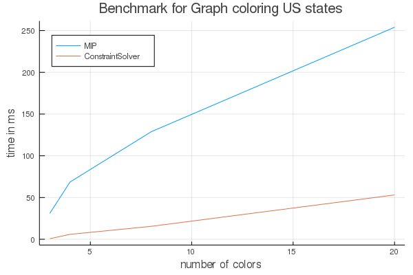
For every color the MIP needs more constraints which makes it slower from time to time. The constraint solver saves information for each tree node even if we don't visit that node later. This slows down sorting of the nodes and maybe some other things.
What's next?
There are some thins missing:
More objective function possibilities
If we found a solution and improve on it because the best bound was not achieved we have to jump to that later. I left it out for now
Avoid to many jumps between nodes maybe if prune and reverse prune take too much time.
More test cases bigger colorings (probably not just maps so that we need actually more than 4 colors)
Stay tuned ;)
Next post is out: Documentation & Benchmarks
And as always:
Thanks for reading and special thanks to my first three patrons!
List of patrons paying more than 2$ per month:
Site Wang
Gurvesh Sanghera
I'm very happy for the support I get via Patreon and comments on reddit, HackerNews and Twitter. Would like to make this blog faster as the CMS doesn't turn out to be the best. When I reach my next goal of 50$ per month I'll create a faster blog which will also have a better layout:
Code which I refer to on the side
Code diffs for changes
Easier navigation with Series like Simplex and Constraint Programming
instead of having X constraint programming posts on the home page
And more
If you have ideas => Please contact me!
If you want to support me and this blog please consider a donation via Patreon to keep this project running.
For a donation of a single dollar per month you get early access to the posts. Try it out for the last two weeks of October for free and if you don't enjoy it just cancel your subscription.
If you have any questions, comments or improvements on the way I code or write please comment here and or write me a mail o.kroeger@opensourc.es and for code feel free to open a PR on GitHub ConstraintSolver.jl
I'll keep you updated on Twitter OpenSourcES as well as my more personal one: Twitter Wikunia_de
Want to be updated? Consider subscribing on Patreon for free
