Constraint Solver Part 10: Graph Coloring Part 1
Creation date: 2019-10-10

Series: Constraint Solver in Julia
This is part 10 of the series about: How to build a Constraint Programming solver?
In this post I'll first make a small update to the sum constraint as it should simplify things like 2x+3x to 5x and also 2x-3y+5 == z by moving the 5 to the rhs and the z to the left.
In the second part of this post we create the not equal constraint and use it for graph coloring as I'm missing some visualizations in this series.
Sum Constraint
This time I want to do test driven development that means we define the tests first.
Inside test/small_special_tests.jl:
@testset "Reordering sum constraint" begin
    com = CS.init()

    x = CS.addVar!(com, 0, 9)
    y = CS.addVar!(com, 0, 9)
    z = CS.addVar!(com, 0, 9)

    CS.add_constraint!(com, 2x+3x == 5)
    CS.add_constraint!(com, 2x-3y+6+x == z)
    CS.add_constraint!(com, x+2 == z)
    CS.add_constraint!(com, z-2 == x)
    CS.add_constraint!(com, 2x+x == z+3y-6)

    status = CS.solve!(com)
    @test status == :Solved
    @test CS.isfixed(x) && CS.value(x) == 1
    @test 2*CS.value(x)-3*CS.value(y)+6+CS.value(x) == CS.value(z)
    @test CS.value(x)+2 == CS.value(z)
end
It's important that we test for + and - and single variables as well as LinearVariables and a bit more on the rhs.
then we can run ] test ConstraintSolver
MethodError: no method matching +(::ConstraintSolver.LinearVariables, ::Int64)
That is part of the second constraint as the first one can actually be solved currently but is not converted to a simplified form.
I want that 2x+3x == 5 actually creates the same as 5x == 5.
Therefore I add:
@test length(c1.indices) == 1
@test c1.indices[1] == 1
@test c1.coeffs[1] == 5
@test c1.rhs == 5
to the test case which fails.
Now we can simplify it because we have the same variable index inside the constraint indices or linear variables indices.
At which step do we want to simplify?
We could simplify in + when we build the linear variables object or in == when we actually construct the constraint. I'm going for the latter one as this has overhead only once.
The idea is to sort the indices and if two indices are the same then we add up the coefficients.
This will be done in src/eq_sum.jl but we want to do it later also for <= and >= therefore the function of simplification will be in src/linearcombination.jl.
The new == function:
function Base.:(==)(x::LinearVariables, y::Int)
    lc = LinearConstraint()
    indices, coeffs = simplify(x)
    lc.fct = eq_sum
    lc.indices = indices
    lc.coeffs = coeffs
    lc.operator = :(==)
    lc.rhs = y
    return lc
end
The simplify function:
function simplify(x::LinearVariables)
    set_indices = Set(x.indices)
    # if unique
    if length(set_indices) == length(x.indices)
        return x.indices, x.coeffs
    end

    perm = sortperm(x.indices)
    x.indices = x.indices[perm]
    x.coeffs = x.coeffs[perm]
    indices = Int[x.indices[1]]
    coeffs = Int[x.coeffs[1]]

    last_idx = x.indices[1]
    for i=2:length(x.indices)
        if x.indices[i] == last_idx
            coeffs[end] += x.coeffs[i]
        else
            last_idx = x.indices[i]
            push!(indices, x.indices[i])
            push!(coeffs, x.coeffs[i])
        end
    end
    return indices, coeffs
end
First we check whether the indices are all unique. If yes => don't need to do anything.
Otherwise we sort the indices and coefficients by the indices and create a new output indices, coeffs. For each index we check whether it is the same as the last one and if yes, we add the coeffs otherwise we simply add the index and coeffs to the corresponding arrays and set last_idx.
Now we need to support +(::ConstraintSolver.LinearVariables, ::Int64) I'll do this by using 0 as the index for numbers and the number itself is the coefficient.
function Base.:+(x::LinearVariables, y::Int)
    lv = LinearVariables(x.indices, x.coeffs)
    push!(lv.indices, 0)
    push!(lv.coeffs, y)
    return lv
end
Now I don't want to write a function for x+y == z and x+y == 2+z as the first one is LinearVariables == Variable and the second is LinearVariables == LinearVariables. Therefore I convert the first into the second. The same is true for 2x + 5 and x+5:
function Base.:+(x::Variable, y::Int)
    return LinearVariables([x.idx], [1])+y
end
function Base.:(==)(x::LinearVariables, y::Variable)
return x == LinearVariables([y.idx], [1])
endand now the actual function. Now it looks reasonable to change the simplify function a little bit by also returning a constant left hand side. So whenever there is a 0 in indices it is actually a constant value and we want to move it to the right later.
The first part which is used when an index isn't used more than once gets changed to:
# if unique
if length(set_indices) == length(x.indices)
    if 0 in set_indices
        indices = Int[]
        coeffs = Int[]
        lhs = 0
        for i=1:length(x.indices)
            if x.indices[i] == 0
                lhs = x.coeffs[i]
            else
                push!(indices, x.indices[i])
                push!(coeffs, x.coeffs[i])
            end
        end
        return indices, coeffs, lhs
    else
        return x.indices, x.coeffs, 0
    end
end
and the end of the function:
lhs = 0
if indices[1] == 0
    lhs = coeffs[1]
    indices = indices[2:end]
    coeffs = coeffs[2:end]
end

return indices, coeffs, lhs
In the normal == we now have to subtract lhs from y:
function Base.:(==)(x::LinearVariables, y::Int)
    ...
    indices, coeffs, constant_lhs = simplify(x)
    ...
    lc.rhs = y-constant_lhs
    return lc
end
Now back to LinearVariables == LinearVariables.
function Base.:(==)(x::LinearVariables, y::LinearVariables)
    return x-y == 0
end
That was simple. What are we missing?
Let's run the test case: ] test ConstraintSolver.
MethodError: no method matching -(::ConstraintSolver.Variable, ::Int64)Okay that is the same as plus.
function Base.:-(x::Variable, y::Int)
    return LinearVariables([x.idx], [1])-y
end

function Base.:-(x::LinearVariables, y::Int)
    return x+(-y)
end
Let's create a new branch and push it to see whether we have a test for everything we coded. It might be the case that I forgot a test case and also some coding but with codecov we can at least see whether there is a test missing which we actually coded.
I called it feature-combined-sums and as I actually have an issue #15 for it we should put #15 in our commit message such that it gets linked.
Pushing and creating a pull request:
Okay after a while I decided that Travis is sometimes just too slow for me and GitHub Actions seems to be faster. So I included codecov into GitHub Actions and removed travis:
the new GitHub Actions file: main.yml
name: Run tests

on: [push, pull_request]

jobs:
  test:
    runs-on: ${{ matrix.os }}
    strategy:
      matrix:
        julia-version: [1.0.4, 1.2.0]
        julia-arch: [x64]
        os: [ubuntu-latest, windows-latest, macOS-latest]

    steps:
      - uses: actions/checkout@v1.0.0
      - name: "Set up Julia"
        uses: julia-actions/setup-julia@v0.2
        with:
          version: ${{ matrix.julia-version }}
          arch: ${{ matrix.julia-arch }}
      - name: "Build package"
        uses: julia-actions/julia-buildpkg@master
      - name: "Run tests"
        uses: julia-actions/julia-runtest@master
      - name: "CodeCov"
        uses: julia-actions/julia-uploadcodecov@master
        env:
          CODECOV_TOKEN: ${{ secrets.CODECOV_TOKEN }}
you get the CODECOV_TOKEN in the settings of codecov and then need to add it to the secret keys of your GitHub project.
Oh everything went fine and we have 100% diff coverage.
Graph Coloring
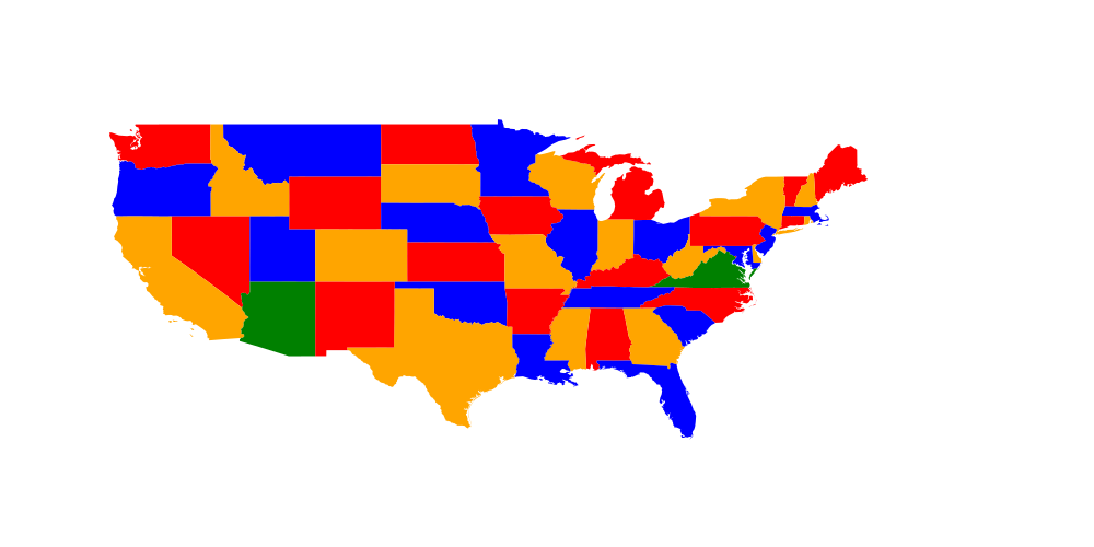
What do we want to do?
We want to color the US states in such a way that two states don't have the same color. As it is a map we know that we need at most 4 colors. That means we can have 49 (I removed Alaska and Hawaii but D.C. is included) variables each with the possibilities 1,2,3 and 4. We just have to create the not equal constraint.
Why only four colors?
In that video Dr. James Grime gives a good idea about why four colors are enough without giving the full prove but I think the idea is very valuable.
In the upcoming posts I will introduce the option to get all solutions which might be interesting for Sudoku for example if people want to create a sudoku instead of solving it by generating some numbers and check whether that is sufficient to make it unique. I'll also add the functionality to optimize i.e the maximum color should be minimized. That is a bit more complicated I think but we'll get there.
First of all let us solve the simplest version of graph coloring using this map.
We just have to introduce the constraints which is a list of != constraints like
CS.add_constraint!(com, washington != oregon)
CS.add_constraint!(com, washington != idaho)
after we introduced all the variables we need like:
washington = CS.addVar!(com, 1, 4)
montana = CS.addVar!(com, 1, 4)
Implementing the != constraint. One might think we can use the same technique as before by introducing:
function Base.:(!=)(x::Variable, y::Variable)
    bc = BasicConstraint()
    bc.fct = not_equal
    bc.indices = Int[x.idx, y.idx]
    return bc
end
in src/not_equal.jl (new file). Unfortunately this doesn't work because the != doesn't work as it is interpreted as !(x == y). Therefore we have to use something like this:
function Base.:!(bc::CS.BasicConstraint)
    if bc.fct != equal
        throw("!BasicConstraint is only implemented for !equal")
    end
    if length(bc.indices) != 2
        throw("!BasicConstraint is only implemented for !equal with exactly 2 variables")
    end
    bc.fct = not_equal
    return bc
end
So we create the equal constraint first and then we change it to a not equal one.
We of course create a
function not_equal(com::CS.CoM, constraint::BasicConstraint; logs = true)function as well were we have our basics at the top:
indices = constraint.indices

changed = Dict{Int, Bool}()
pruned  = zeros(Int, length(indices))
pruned_below  = zeros(Int, length(indices))

search_space = com.search_space
and then as we always have exactly two variables we write.
v1 = search_space[indices[1]]
v2 = search_space[indices[2]]
fixed_v1 = isfixed(v1)
fixed_v2 = isfixed(v2)
if !fixed_v1 && !fixed_v2
    return ConstraintOutput(true, changed, pruned, pruned_below)
elseif fixed_v1 && fixed_v2
    if value(v1) == value(v2)
        return ConstraintOutput(false, changed, pruned, pruned_below)
    end
    return ConstraintOutput(true, changed, pruned, pruned_below)
end
that checks whether exactly one of the variables is set. If that is not the case we can return as it's either infeasible or we can't reduce the search space.
If one is fixed we can remove the value from the other one if it has the value:
# one is fixed and one isn't
if fixed_v1
    prune_v = v2
    prune_v_idx = 2
    other_val = value(v1)
else
    prune_v = v1
    prune_v_idx = 1
    other_val = value(v2)
end
if has(prune_v, other_val)
    if !rm!(com, prune_v, other_val)
        return ConstraintOutput(false, changed, pruned, pruned_below)
    end
    changed[indices[prune_v_idx]] = true
    pruned[prune_v_idx] = 1
end
return ConstraintOutput(true, changed, pruned, pruned_below)
and the third part of src/not_equal.jl is again to check whether it's feasible if we set a value in backtracking.
function not_equal(com::CoM, constraint::Constraint, value::Int, index::Int)
    if index == constraint.indices[1]
        other_var = com.search_space[constraint.indices[2]]
    else
        other_var = com.search_space[constraint.indices[1]]
    end
    return !issetto(other_var, value)
end
That is it!
But it's probably not that interesting to see the end result. We would like to visualize how the solver found it out.
Not sure how to visualize it such that one can see the current search space :/ What I can show you for now is the value currently fixed which might get changed in backtracking. (Here it isn't)

The reason why there is no change sometimes is when pruning a value but I find it interesting to get an idea of how many pruning steps there are before the next fix.
Let's have a look which got fixed by pruning (black circle) and which got fixed by trying out (white circle).

In general we can see that we used a lot of free choices and didn't prune often.
I think it might be more interesting to see what happens if we limit the number of colors to 3.

There one can see a problem of using my strategy of setting a variable which was infeasible most often before in backtracking even though it works quite nicely in sudoku. Another thing is: If we set Washington to red and it doesn't work then setting it to blue doesn't work as well because we could always swap colors in the whole map i.e all which were blue are now red and vice versa. That doesn't change any constraint.
What's next?
Optimization function i.e use as few colors as possible done
Speed up: Reduce vector allocation when we use only two variables
Yes probably changing the data structure again. It's work in progress ;)
also done
Stay tuned ;)
And as always:
Thanks for reading and special thanks to my first three patrons!
List of patrons paying more than 2$ per month:
Site Wang
If you want to have early access to the next posts as well and enjoy the blog in general please consider a donation via Patreon to keep this project running.
For a donation of a single dollar per month you get early access to the posts. Try it out for a the last two weeks of October for free and if you don't enjoy it just cancel your subscription.
If you have any questions, comments or improvements on the way I code or write please comment here and or write me a mail o.kroeger@opensourc.es and for code feel free to open a PR on GitHub ConstraintSolver.jl
I'll keep you updated on Twitter OpenSourcES as well as my more personal one: Twitter Wikunia_de
Want to be updated? Consider subscribing on Patreon for free
