Javis v0.3: How to animate a Fourier series
Creation date: 2020-11-12

It's been a while since we released v0.2 of Javis and that I have posted about it here.
In that post I gave a view about the potential future of Javis. We finally released v0.3 and the future is now the default.
Just listing all the changes we made would probably be quite boring and therefore I want to create a neat animation along the way and explain some parts of the awesome Fourier series.
I think quite a lot of people have heard about the Fourier series but didn't fully understand it. I'm quite sure I'm still part of that crew. Others might not know what I'm talking about and I don't know whether it's a good idea to read this post as your introduction but I'll give my best.
Additionally, I envy the latter group because Fourier series is something extremely fascinating.
This blog is mostly for readers who are interested in Javis and JuliaLang so I'll start with the changes we did for v0.3.
Changes in v0.3 on a higher level
We finally have a version for transposing a matrix or I prefer to say general morphing capabilities as transposing only works sometimes 😄 Nevertheless, I'll make a post about that shortly after this one. (Okay let's say in November... hopefully)
Something that unfortunately didn't make it into v0.3 though is the ability to have layers but we are getting there. We conceptually have a plan for it but haven't found the time to code it yet. There might be also some tweaks to the concept.
The next point from the list of the previous post is "Renaming stuff".
We did rename quite a few things and I hope a bit that you either haven't used v0.2 of Javis 😂 OR that you are adaptable and are happy with the changes we made.
Let's just list a few of them:
Action and SubAction are now called Object and Action respectively. This is due to the fact that the Action before describes more the object itself and doesn't have the capability to actually move the object now. It had the option before but we decided to remove it. We did this to simplify the codebase and make the distinction much clearer.
Next up we simplified BackgroundAction to Background. No more comments on that 😄
Finally we removed Translation, Rotation and Scaling and introduced anim_translate, anim_rotate/anim_rotate_around as well as anim_scale because working with functions instead of structs seems to be more natural and the naming specifies that we do some animation here and not a static translation.
Our last mayor change was to get rid of the javis function and the weird design I started with. It was a huge mess with these weird arrays.
One now defines the video, objects and actions just line by line and renders the video in the end.
Just to give you an example
using Javis
function ground(args...)
    background("black")
    sethue("white")
end

video = Video(800, 400)
Background(1:100, ground)
ball = Object((args...)->circle(O, 100, :fill), Point(-500, 0))
rolling = Action(anim_translate(Point(1000, 0)))
act!(ball, rolling)

render(video; pathname="rolling_ball.gif")
I think one can clearly see what is defined where besides maybe a few quirks... 😄
The circle function takes the center point and the radius as well as the action (here :fill). Why do I define it at the center center? I could have defined it at Point(-500, 0) but I like to think of objects being centered and then move them around. Maybe it's just me but it has the advantage that it's easy to scale objects correctly and makes rotations easier.
It's not really possible to see a rotation of a circle (currently we don't rotate it). How about adding something to the circle such that we can differentiate between a rotating circle and a moving one.
using Javis
function ground(args...)
    background("black")
    sethue("white")
end

function my_circle(args...)
    circle(O, 100, :fill)
    sethue("black")
    line(O, Point(100, 0), :stroke)
end

video = Video(800, 400)
Background(1:100, ground)
ball = Object(my_circle, Point(-500, 0))
translating = Action(anim_translate(Point(1000, 0)))
rotating = Action(anim_rotate(0.0, 2*2π))
act!(ball, [translating, rotating])

render(video; pathname="rolling_ball_2.gif")
That one is clearly rolling. Okay I might have gotten a bit distracted with that one 😄 but we can reuse that for later.
Now in v0.2 it would be quite hard to make the line inside the circle grow longer with time I think. Actually this was possible with v0.2.2 but I haven't written about it yet so this is the time of change.
using Javis
function ground(args...)
    background("black")
    sethue("white")
end

function my_circle(args...; line_length=0)
    circle(O, 100, :fill)
    sethue("black")
    setline(2)
    line(O, Point(line_length, 0), :stroke)
end

video = Video(800, 400)
Background(1:100, ground)
ball = Object(my_circle, Point(-500, 0))
translating = Action(anim_translate(Point(1000, 0)))
rotating = Action(anim_rotate(0.0, 2*2π))
changing_len = Action(change(:line_length, 0 => 100))
act!(ball, [translating, rotating, changing_len])

render(video; pathname="rolling_ball_3.gif")
It's now finally possible to simply change values in an animated way directly.
We kind of have the building blocks for fourier now 😉
Fourier series
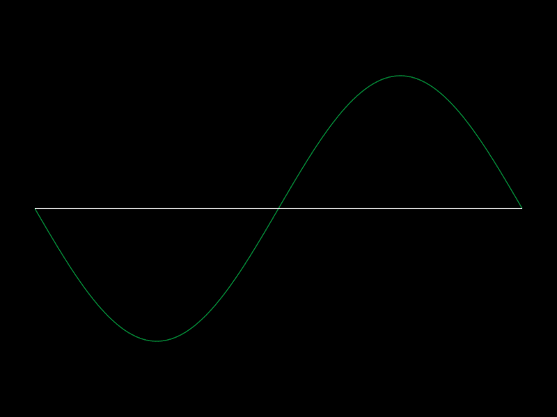
In simple words we try to combine simple things to create everything.
Like combining sine waves by addition to create/approximate every function.
How about the square function as an example?
The Code
using Javis, Colors
function ground(args...)
    background("black")
    sethue("white")
    translate(-args[1].width/2+50, 0)
    scale(700, 150)
end

function wave(xs, ys, opacity, color)
    setline(1.5)
    setopacity(opacity)
    sethue(color)
    points = Vector{Point}(undef, length(xs))
    for (x, y, i) in zip(xs, ys, 1:length(xs))
        points[i] = Point(x, y)
    end
    prettypoly(points, :stroke, ()->())
end

function term(x, i)
    return 4/π * sin.(2π*(2i-1)*x)/(2i-1)
end

function sum_term(x, k)
    k == 0 && return zeros(length(x))
    return sum(term(x, i) for i in 1:k)
end

nframes = 300
frames_per_wave = 40
video = Video(800, 600)
Background(1:nframes, ground)

x = 0.0:0.001:1.0
k = 6
colors = [RGB(0.0, 1.0, 0.4), RGB(0, 1.0, 1.0), RGB(1.0, 0.25, 0.25), RGB(1.0, 1.0, 0.0), RGB(1.0, 0.5, 1.0), RGB(0.75, 0.75, 1.0)]
waves = Object[]
for i = 1:k
    frames = frames_per_wave*(i-1)+1:nframes
    push!(waves, Object(frames, (args...; y=term(x,i)) -> wave(x, y, 0.5, colors[i])))
    act!(waves[end], Action(5:frames_per_wave,
                    change(:y, term(x,i) => sum_term(x, i))))
end

sum_wave = Object(1:nframes, (args...; y=zeros(length(x)))->wave(x, y, 1.0, "white"))
for i = 1:k
    act!(sum_wave, Action(frames_per_wave*(i-1)+1:frames_per_wave*i,
                         change(:y, sum_term(x, i-1) => sum_term(x, i))))
end

render(video; pathname="images/fourier_1D.gif")
We basically try to combine simple waves (sine waves) and add them up to create a square wave.
Importantly there is nothing special about the square function. This works with every function. One just needs to add quite a lot of the functions together. For the actual result we need infinitely many.
Let's quickly change to 2D
I actually want to draw something in 2D though instead of this 1D function. 2D is much more interesting when you ask me.
BTW this entire idea of using Javis to visualize the Fourier series came from Riccardo Cioffi, who I like to call the first user of Javis. He also coded it himself without us knowing about this until we saw his post about it on the JuliaLang discourse. Please check it out!
It was done using a previous version of Javis so the code doesn't work anymore.
I'll wait here for a couple of minutes while you enjoy his stunning visualization.
Let's start with some building blocks that make sense to understand the Fourier series in 2D. I'll start with circles and complex numbers.
In general I'll basically go through the stuff that Grant Sanderson explained beautifully on his YouTube Channel 3blue1brown But what is a Fourier series?. There are some more references at the end of this post 😉
You've seen some circles before but let's have a look at how to work with them using complex numbers.
I here refer to the usage of the formula
\[ e^{2\pi i t} \]where t is our variable ranging from 0 to 1 and i is the imaginary unit.
This therefore computes a complex number when we give it some \(t\). We plot that by simply using the real component of our complex number on the x-axis and the complex component on the y-axis.
In this visualization the circle is drawn up to a certain point at each frame and completes the circle with t=1.00

This is just something to keep in mind for the rest of the post.
Next up we start with a shape let's say a star that we want to draw using circles rotating around circles as circles are the sine waves of 2D space.
I think this is best explained visually so I'll show you what we are trying to achieve first and then show you how to get there.
What we want to create
This is kind of what we want to achieve but we will have a look at more complicated shapes later. For that we will use more circles though and then it's hard to grasp what's going on.
The code for those of you who are interested
using Javis, FFTW, FFTViews

function ground(args...)
    background("black")
    sethue("white")
end

function circ(; r = 10, vec = O, action = :stroke, color = "white")
    sethue(color)
    circle(O, r, action)
    my_arrow(O, vec)
    return vec
end

function my_arrow(start_pos, end_pos)
    start_pos ≈ end_pos && return end_pos
    arrow(
        start_pos,
        end_pos;
        linewidth = distance(start_pos, end_pos) / 100,
        arrowheadlength = 7,
    )
    return end_pos
end

function draw_line(
    p1 = O,
    p2 = O;
    color = "white",
    action = :stroke,
    edge = "solid",
    linewidth = 3,
)
    sethue(color)
    setdash(edge)
    setline(linewidth)
    line(p1, p2, action)
end

function draw_path!(path, pos, color)
    sethue(color)

    push!(path, pos)
    draw_line.(path[2:end], path[1:(end - 1)]; color = color)
end

function get_points(npoints, options)
    Drawing()
    shape = poly([Point(-200, 0), Point(250, 70), Point(165, -210)]; close=true)
    points = [Javis.get_polypoint_at(shape, i / (npoints-1)) for i in 0:(npoints-1)]
    return points
end

function poly_color(points, action; color=nothing)
    color !== nothing && sethue(color)
    poly(points, action)
end

c2p(c::Complex) = Point(real(c), imag(c))

remap_idx(i::Int) = (-1)^i * floor(Int, i / 2)
remap_inv(n::Int) = 2n * sign(n) - 1 * (n > 0)

function animate_fourier(options)
    npoints = options.npoints
    nplay_frames = options.nplay_frames
    nruns = options.nruns
    nframes = nplay_frames + options.nend_frames

    points = get_points(npoints, options)
    npoints = length(points)
    println("#points: $npoints")

    # optain the fft result and scale
    x = [p.x for p in points]
    y = [p.y for p in points]

    fs = fft(complex.(x, y)) |> FFTView
    # normalize the points as fft doesn't normalize
    fs ./= npoints
    npoints = length(fs)

    video = Video(options.width, options.height)
    Background(1:nframes, ground)
    Object((args...)->poly_color(points, :stroke; color="green"))

    circles = Object[]
    npoints = 5

    for i in 1:npoints
        ridx = remap_idx(i)

        push!(circles, Object((args...) -> circ(; r = abs(fs[ridx]), vec = c2p(fs[ridx]))))

        if i > 1
            # translate to the tip of the vector of the previous circle
            act!(circles[i], Action(1:1, anim_translate(circles[i - 1])))
        end
        ridx = remap_idx(i)
        act!(circles[i], Action(1:nplay_frames, anim_rotate(0.0, ridx * 2π * nruns)))
    end

    trace_points = Point[]
    Object(1:nframes, (args...) -> draw_path!(trace_points, pos(circles[end]), "red"))

    render(video, pathname = options.filename)
end

function main()
    gif_options = (
        npoints = 1000, # rough number of points for the shape => number of circles
        nplay_frames = 400, # number of frames for the animation of fourier
        nruns = 2, # how often it's drawn
        nend_frames = 0,  # number of frames in the end
        width = 800,
        height = 500,
        shape_scale = 0.8, # scale factor for the logo
        tsp_quality_factor = 40,
        filename = "images/fourier_tri_5.gif",
    )
    animate_fourier(gif_options)
end

main()
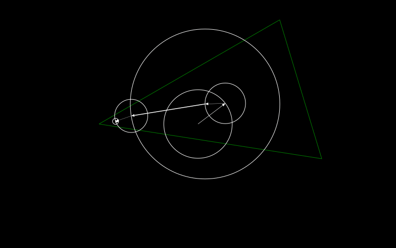
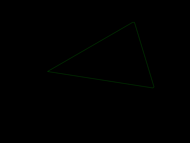
We try here to draw the green triangle by using five circles. They approximate the triangle as you can see with the red shape that gets drawn.
Each circle has a vector attached to it. Let's start from the inner stationary circle where the vector is fixed.
The vector points to the center of the triangle which makes sense as this is the best point to make sure that the balance of the rotating circles around it is not off. I'll also come back to it at the later point of this long long post.
How about the next circle in the chain? It doesn't move but has its center where the last circle pointed to. Additionally the vector inside does rotate now. Here it has a full clockwise rotation for the full drawing.
Now the next three circles do move. The vector inside the next one in the chain has the same speed as the previous circle but runs anti clockwise. The other two do two rotations in one full drawing. One going clockwise the other anti clockwise.
This is kind of all there is to it. Well at least it gives a visualization of what we want to achieve and you might guess already that adding more circles to it makes the approximation better.
How to get there by computing it ourselves
In this section I want to talk a bit about the formula that some of you might have seen before and compute the parameters of the five circles shown above.
\[ \sum_{k=-n}^n c_k e^{k\cdot 2\pi i t} \]We saw \(e^{2\pi i t}\) before so \(k\) is the only new thing in the exponential part. One can see from the circle animation (where we draw a circle) above that \(k\) basically just defines the speed and the sign of \(k\) the rotation direction.
This means we have our non rotating circle with \(k=0\) and our rotating circles with \(k \in \{-1, 1, -2, 2\}\) from before. The only thing left is the \(c_k\).
\(c_k\) needs to define the radius of the circle which is easy with a number like \(2.5\) or \(0.5\) to have a radius of 2.5 or 0.5. Additionally it has to define the starting rotation of the circle. This is basically what the vector inside of it is indicating. We had a look at complex numbers before a bit and when defining \(c_k\) as a complex number we have exactly these two pieces of information given by the absolute value and the angle of the complex number.
Let's have a look at the components for \(n=1\):
\[ c_{-1} e^{-2\pi i t} + c_{0} e^{0\cdot 2\pi i t} + c_{1} e^{2\pi i t} \]which can be simplified by using \(e^0 = 1\) to:
\[ c_{-1} e^{-2\pi i t} + c_{0} + c_{1} e^{2\pi i t} \]What does happen if we take the average of this when we let \(t\) move from \(0\) to \(1\) so draw the full circles?
First of all we can compute the average of the sum by summing up the averages.
If we average the positions of a circle we obtain the center which is at (0,0) for all of them. Therefore, averaging over all possibilities of t between 0 and 1 (or at least a good subset of all possibilities... okay well let's say a few hundred points 😄 instead of infinitely many) we obtain \(c_0\). Isn't that quite nice?
Let's recap that again: We average over the summands and because all the summands besides \(c_0\) are circles they average out to \((0, 0)\) and are irrelevant.
This was also the intuition we got from the result shown with the five circles desperately trying to approximate a triangle.
Well wait and how do we get the \(c_{-1}\) and all the other constants \(c_k\)?
Actually we do exactly the same thing and just multiply the whole equation by \(e^{1\cdot 2\pi i t}\) to obtain a shifted version. Remember that \(e^x \cdot e^y = e^{x+y}\) such that we can cancel out the exponent with this multiplication. By multiplying with \(e^{1\cdot 2\pi i t}\) we cancel out the component we have for \(k=-1\). We can do the same thing for all of the constants.
Let's make a nice visualization for that:
This one might seem a little bit more complicated so let's break it down.
We start with a green triangle
We use 100 points on that triangle and average it out
Create a circle centered at the origin and point to the average using a vector
We multiply the triangle with \(e^{k \cdot 2\pi i t}\) with \(k=-1\) and \(t\) depends on the position we are on the triangle.
Create new 100 points and average them again
Create a new circle
Move the newly created circle to the tip of the previous circle
This can be repeated to obtain all the other constants and therefore circles that we need to add.
Using a package to handle the heavy work
Instead of multiplying and averaging ourselves, we can use a package for that. I hope I could convince everyone who wasn't convinced before that fourier series are quite nice so there is of course much more stuff to it than I explained here or understand myself 😄
There are two nice packages that I used in my fourier triangle animation I showed before.
The first one does the heavy computation and it does it fast so the first "F" in the name stands for fast.
FFTViews on the other hand just makes it easier to work with. As you have seen before we deal with negative and positive values for \(k\).
FFTW produces a vector with all those constants \(c_k\) but FFTViews makes it possible to index that information more naturally with \(c[-3]\) for example even though Julia is a one-index based language.
One inputs the vector of points as a vector of complex numbers. An extra step one needs to perform is to average the result as this isn't done by the algorithm (probably one way to make it faster 😉 )
By average I mean that one needs to divide the result by the number of points.
I would like to close this post by showing a final result I made and a bit of the thing that was needed for it. Afterwards I'll post a link to the code as usual.
The final animation
In that example I also used the travelling salesman problem (TSP) to combine all the letters into one continuous shape.
A short side note:
If you're interested in the travelling salesman problem or optimization in general I highly recommend checking some other posts I've written about it in the past:
Okay back to the post:
We need to use the travelling salesman problem to avoid having big jumps from one letter to another as the drawing is continuous. One can potentially get rid of the jumps all together by having a discontinuous version of the fourier series.
In the code I've linked below I also use the same variable for number of points and circles which isn't the greatest idea and I have change that for the triangle drawing but I wanted to limit the running time of the TSP heuristic solver in this case.
If you want to see how this is done please have a look at this gist
Conclusion
Before I'll end this post with an advertisement for myself 😄, let me summarize a bit what we have learned in the last 20 minutes.
The basic changes of Javis in v0.3
Drawing simple shapes and apply actions to them
What one can do with the fourier series in 1D and 2D
The formula and explanation of the fourier series
An intuition of how to obtain the needed constants
Now there is the advertisement. All of the above is free for everyone to read which is probably not a surprise to you in the times of the world wide web. Nevertheless, it takes quite some time to build the tools and write those posts. If you enjoy at least a couple of those posts on my blog: Please consider subscribing on Patreon for as little as a dollar per month.
I can't even think of how many milliliters of coffee or tea that is per day...
With your subscription you'll get these posts earlier as everyone else!
Special thanks to my 10 patrons!
Special special thanks to my >4$ patrons. The ones I thought couldn't be found 😄
Site Wang
Gurvesh Sanghera
Szymon Bęczkowski
DShiu
For a donation of a single dollar per month you get early access to these posts. Your support will increase the time I can spend on working on this blog.
There is also a special tier if you want to get some help for your own project. You can checkout my mentoring post if you're interested in that and feel free to write me an E-mail if you have questions: o.kroeger <at> opensourc.es
I'll keep you updated on Twitter OpenSourcES.
List of useful resources
Video explanation by 3blue1brown But what is a Fourier series?
Video coding by The Coding Train Coding Challenge: #125 Fourier Series
Blog post at betterexplained.com An Interactive Guide To The Fourier Transform
Want to be updated? Consider subscribing on Patreon for free
