Time for a new post in this Javis Examples Series. Last time we had a look at a problem that we wanted to visualize. This time we just want to create an interesting animation while we are learning about inverse kinematics. It's a topic tackled by a bunch of other bloggers and YouTubers out there already but I hope you'll still enjoy my animated visualizations and the end result in Javis . Maybe you can create your own animations with it 😉

• Inverse Kinematics by The Coding Train

• I Spent a Week Making an AI's Video Game Idea by Sebastian Lague

What is inverse kinematics?

We have a robot arm which consists of several segments. Now we want to grab an object from which we obtained the position for example by computer vision. The question is now how to arrange the segments/which angle to choose at the joints such that the last segment in the arrangement reaches the object.

Fortunately the algorithm for this is rather simple and as you have now seen also very practical.

Explanation by animation

Let me introduce you to the algorithm with a small description and an animation. After that I'll also share the code for the animation with you. As you all know: This is a Javis series 😄

We'll do this with 3 segments for the arm later but it can be however many you want. Let's first assume that we only have one segment though. That might point up at the beginning but the object is to the right. Maybe we make the problem even simpler shall we? Let say we can move the arm around freely so it is not attached to the robot.

Now the solution seems quite simple and obviously there are infinitely many solutions. The head of the segment just needs to be at object and the length of the segment is defined but the start or the angle of the segment can be arbitrarily. However it seems rather helpful to not completely change the angle of the at the moment still upwards pointing segment. Instead we want to change the angle in the direction of the object.

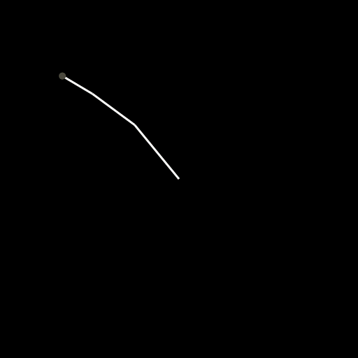
Here you can see one segment of the arm rotating around until it is pointing directly towards the point. Then we just do a simple translation to the point itself. The recursive idea is now to do this for the next segment as well but it doesn't want to reach the object but instead the start of the last segment.

The angle here can be evaluated by using the atan function, which gives us an angle between \(-\pi\) and \(\pi\) when called with two arguments. In other languages this is sometimes called atan2.

We need to call it with: atan(p.y-seg.start.y, p.x-seg.start.x) where \(p\) is the Point we want to reach and seg is our segment with start as its tail.

I'll go into how we make sure that our segment which is attached to the robot doesn't move after the next section. Let's get into the coding part.

Javis basic inverse kinematics

In this section I want to start introducing the basics of the code we need to create a nice little animation for inverse kinematics. Then I'll explain locking the first segment to a point for a stationary robot and also add that part to the implementation.

We start as always with the basics of using Javis and the ground function. Also add a Segment struct.

using Javis

mutable struct Segment 
    start   :: Point 
    angle   :: Float64
    length  :: Float64
    head    :: Point
end

function ground(args...)
    background("black")
    sethue("white")
end

function main()
    vid = Video(512, 512)

    nframes = 200
    Background(1:nframes, ground)

    render(vid; pathname="arm.gif")
end

Each segment just has a start point, an angle, a length and a head point. You only really need two of them or three depending on which one you choose but I found it easier to work with those four 😉

Let's create a single segment first and draw it.

In main:

seg = Segment(O, 0, 100, Point(100, 0))
seg_obj = Object(1:nframes, draw_segment(seg))

and the function:

function draw_segment(seg::Segment)
    @JShape begin
        line(seg.start, seg.head, :stroke)
    end
end

Now we don't want to compute the head all the time if we have the other info so let's create a constructor for Segment and a sethead! function to calculate the missing info.

function Segment(start, angle, length) 
    s = Segment(start, angle, length, O)
    sethead!(s)
    return s
end

function sethead!(seg::Segment)
    dx = cos(seg.angle)*seg.length
    dy = sin(seg.angle)*seg.length
    seg.head = seg.start + Point(dx, dy)
end

function setstart!(seg::Segment)
    dx = cos(seg.angle)*seg.length
    dy = sin(seg.angle)*seg.length
    seg.start = seg.head - Point(dx, dy)
end

then we can use

seg = Segment(O, 0, 100)

I've also added setstart! just that we have a function for the other way around.

Now let's start with the actual code. We want to have a reach! function which does take a segment and a point and rotates the segment towards the point and translate to reach it in the end.

function reach!(seg::Segment, p::Point)
    sethead!(seg)
    seg.angle = atan(p.y-seg.start.y, p.x-seg.start.x)
    seg.head = p
    setstart!(seg)
end

Here we make sure to compute the head from the given info. Then we compute the angle using the atan function as discussed before. The translation is done by simply fixing the head to p and then call the setstart! function.

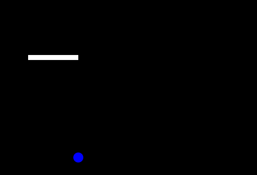
Now if we call reach!(seg, Point(100, 100)) before calling the Object we would get this:

I've also added this to show the object itself:

Object(1:nframes, JCircle(Point(100, 100), 5; color="blue", action=:fill))

You might want to check out the JCircle function which is relatively new to Javis. You can specify the position, radius the color and whether it should be filled or just outlined (:stroke)

Before we add more segments let's do a little bit of animation with what we have by moving the point.

We need to call the reach! function for this inside the draw_segment function and pass a point to it and be able to change it with change .

function draw_segment(seg::Segment, p::Point)
    @JShape begin
        reach!(seg, p)
        line(seg.start, seg.head, :stroke)
    end p=p
end

The p=p at the end of @JShape makes it possible to change the p later using change .

Now let's change the p in a continuous fashion with:

p = Point(100, 100)
seg_obj = Object(1:nframes, draw_segment(seg, p))
obj = Object(1:nframes, JCircle(Point(100, 100), 5; color="blue", action=:fill))
act!(seg_obj, Action(1:nframes, change(:p, p => Point(190, 20))))
act!(obj, Action(1:nframes, change(:center, p => Point(190, 20))))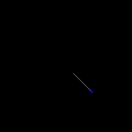

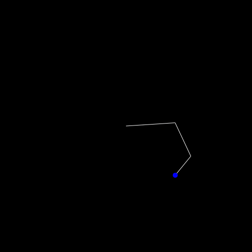
More segments!

Okay let's do this! One segment is boring, isn't it? Let's add some more to see it in action. First we change seg = Segment(O, 0, 100) to segs = [Segment(O, 0, 100), Segment(Point(100,0), 0, 75), Segment(Point(175,0), 0, 50)]

Then we also pass segs to the draw_segment function and while we are at it: Maybe rename it to draw_arm. Don't worry I'll share the whole code at the end of the post 😉

The main change for this besides also drawing the segments in the for loop is the creation of this function:

function reach!(arm::Vector{Segment}, p::Point)
    for i in length(arm):-1:1
        reach!(arm[i], p)
        p = arm[i].start
    end
end

We start with the last segment and call the old reach! function on the initial point. Then we change the point to the start of the newly placed segment and go down in the list of segments.

You can see in the animation above though that the base of the arm isn't stationary though. If we can move the robot itself in the two dimensions we have, why do we even need an arm then? 😄

Let's fix that in the next section. It's simpler than you might think.

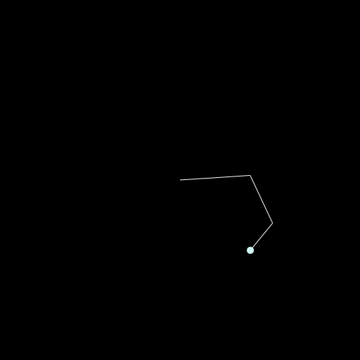
Locking the base!

I said it's simpler than you think but let me start with something that is even simpler than it actually is 😄

We simply do all the stuff we did before and then move the base of the arm to where it should be.

Yeah that is mostly it but as you can imagine it can't really work because if we move it to that place and all segments attached to it, the hand (last segment which grabs the object... am I really explaining what a hand is? 😄 ) will actually not grab the object anymore but it turns out that once the base is actually at the locked position we are always quite close to the target. (Given that the length of the arm is long enough).

What we can do to actually grab the object is the following: Iteration! Basically just doing the same thing over and over again until we are in a given error margin.

There is probably a better way to write this but I've changed the reach! function to this:

function reach!(arm::Vector{Segment}, p::Point)
    end_point = p 
    locked_point = arm[1].start
    loop = false
    if distance(locked_point, end_point) <= sum(s->s.length, arm)
        loop = true
    end
    loop_counter = 0
    while loop_counter == 0 || loop
        p = end_point
        for i in length(arm):-1:1
            reach!(arm[i], p)
            p = arm[i].start
        end
        # move the arm back 
        arm[1].start = locked_point
        sethead!(arm[1])
        for i in 2:length(arm)
            arm[i].start = arm[i-1].head
            sethead!(arm[i])
        end

        # check such that we don't get into an infinite loop or are already close enough
        loop_counter += 1
        if loop_counter == 10 || distance(end_point, arm[end].head) <= 0.1
            break
        end
    end
end

First we save the point we want to reach and the locked point of the base. Then we check whether we can reach the point by just computing whether the arm is long enough. If that isn't the case we only want to run the inner call ones, as we still want point into the right direction.

Then we do our normal reaching stuff and then in # move the arm back we set the start of our first segment and the head and do that for the remaining segments such that they are all connected.

At the end we check whether we reached our goal or whether we have to go into a second/third/... loop. We don't want to get stuck in an infinite loop so I've set the break point after 10 calculations.

Now we know all we need to know to create stunning animations using inverse kinematics.

Hilbert curves and color

My idea was the following: I want to somehow see the different angles of the three segments as a color and let the robot more or less paint something. I think moving line by line or column by column isn't very interesting therefore I decided to use space filling curves like the Hilbert Curve.

Let's maybe start with not moving the object but instead create a circle at each frame which stays there.

For this I simply added the following to the draw_arm function and also created an empty vector points before creating the Object . You can read more about this in our first Javis tutorial.

push!(points, segs[end].head)
sethue("blue")
for point in points
    circle(point, 5, :fill)
end

Making them all blue is probably a bit lame so let's create a struct ColoredPoint.

struct ColoredPoint
    p :: Point 
    c :: HSL{Float64}
end

for the colorspace HSL we need using Colors.

Then we get the color with something like this:

function get_color(arm::Vector{Segment})
    an = [(seg.angle+π)/2π for seg in arm]
    return HSL(an[1]*360, an[2], an[3]*0.8+0.2)
end

Feel free to create your own version with this. The first line here is to have a normalized vector from 0 to 1 of the angles.

The idea is to compute the color based on the angles and instead of storing the Point vector as above we will have a ColoredPoint vector and draw by calling sethue with the specified color.

Now the last step is to create the Hilbert curve. For this I used the package: HilbertSpaceFillingCurve which is rather old but still functional.

It has the function hilbert(d::T, ndims, nbits = 32) where d is basically the index ranging from 0 to (2^nbits)^ndims-1. It will give you back a vector of ndims dimensions and a part of a coordinate is in the range of 0 to 2^nbits-1. Maybe it will be clearer in our specific example. I choose the dimensions of the image as 512x512 which means each dimension is 2^9 such that we can set nbits = 9. Now we want to fill the whole space which means we have 512^2 values for the index d which is over 250,000. I don't want to have that many frames such that I decided to have 2000 frames which is a bit over one minute for 30fps. And just step over a couple of indices to not actually fill the complete space 😄

Well that was kinda unexpected 😂 Well it seems like the arm isn't long enough but as a matter of fact: I like this one even more than the square one I created before so I leave it like that.

I don't want to bother you with the last implementation details as you can find the whole code here but I think the last thing I wanna mention is that you can use Animations to define the transitions of one point to another and pass it over to the change function like this:

anim_p = Animation(
    [i/(length(ps)-1) for i in 0:length(ps)-1], # must go from 0 to 1
    ps,
    [linear() for _ in 1:length(ps)-1],
)

act!(arm_obj, Action(1:nframes, anim_p, change(:p)))

In this case the ps are the points created by hilbert and we don't really need the transitions as we jump from one to another in one frame but it's still easier to pass it to the change function this way.

Alrighty! Thanks everyone for checking out my blog again and see you soon!

And don't forget to subscribe to my free email newsletter to not miss a post.

Or well you can go one step further if you have some money to spare 😉

Thanks to my 12 patrons!

Special special thanks to my >4$ patrons. The ones I thought couldn't be found 😄

• Anonymous

• Kangpyo

• Gurvesh Sanghera

• Szymon Bęczkowski

• Håkan Kjellerstrand

• Colin Phillips

• Jérémie Knuesel

For a donation of a single dollar per month you get early access to these posts. Your support will increase the time I can spend on working on this blog.

There is also a special tier if you want to get some help for your own project. You can checkout my mentoring post if you're interested in that and feel free to write me an E-mail if you have questions: o.kroeger <at> opensourc.es

I'll keep you updated on Twitter OpenSourcES.

atan(y)
atan(y, x)

julia> rad2deg(atan(-1/√3))
-30.000000000000004

julia> rad2deg(atan(-1, √3))
-30.000000000000004

julia> rad2deg(atan(1, -√3))
150.0

Object

1. JCircle(center::Point, radius::Real; kwargs...)
2. JCircle(center_x::Real, center_y::Real, radius::Real; kwargs...)
3. JCircle(p1::Point, p2::Point; kwargs...)
    - A circle that touches `p1` and `p2`
4. JCircle(radius::Real)
    - A circle at the origin

change(s::Symbol, [val(s)])

Background(1:100, ground)
obj = Object((args...; radius = 25, color="red") -> object(O, radius, color), Point(100, 0))
act!(obj, Action(1:50, change(:radius, 25 => 0)))
act!(Action(51:100, change(:radius, 0 => 25)))
act!(Action(51:100, change(:color, "blue")))

@JShape(body, args...)

Object(@JShape begin
    sethue(color)
    poly(points, action, close = true)
end action = :stroke color = "red" radius = 8)

sethue("black")
sethue(0.3, 0.7, 0.9)
setcolor(sethue("red")..., .2)