Kaggle Santa 2019: Final take
Creation date: 2020-01-27

My final steps during the competition
Before I go over the optimal solution, which I only found because I read what other teams did after the competition ended, I want to go briefly over the things I didn't talk about in my last two posts about the challenge:
There is not much more to add to the swapping part from the last post besides some things I encountered. In the following a,b,c are family ids and A,B,C are the days they currently visit the workshop.
Swaps of the form a->B, b->C, c->A didn't work as well as a->B, b->C, c->D
this is normal as the last c->A normally destroys it
How did I choose a,b,c? + d,e,... for longer swap patterns?
a is chosen from randomly from the 5000 families
b is chosen by choosing B as a day of the choices from a
and then b is chosen randomly
this continues til the end
I reject the current set if I chosen the same family more than once
For performance reasons:
I precompute the days and choices for each family and update the assigned day after I make a change. (Probably everyone does that)
Only compute the resulting change in costs
Easy for preference cost
Bit harder for preference costs
=> In the end I had about 1 million swaps per second on my machine.
In general I experimented a lot with the temperature in simulated annealing and with falling back to previous solutions when stuck which were quite helpful but I explained the interesting stuff in the last post.
Let's move from swapping to the MIP approach. Last time I mentioned a way to find the optimal arrangement if we know how many people visit the workshop per day.
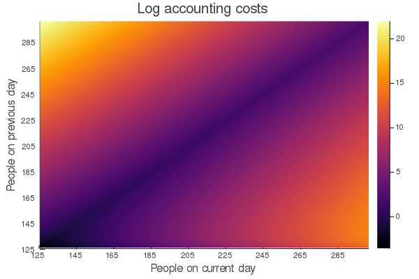
Which we normally don't know :D Therefore that was quite pointless. We want to get the optimal solution without knowing how many people are visiting each day which is much harder. Therefore we need to change the objective function to take the accounting costs into consideration. This is normally not really possible as the accounting costs are not linear but we can linearize them by precomputing all combinations beforehand which means the basically the graph I showed last time:
I tried to work with the number of people on the current day and the difference to the next day but this doesn't make anything easier but more complicated and I wasn't able to achieve good results with it in the end. I'm still not completely sure why this was worse than the approach I used afterwards but okay... So what did I use? Pretty much just what was published in the discussion forum.
That means in a bit of julia code (leaving some things out for simplicity):
n_families = 5000
MIN_OCCUPANCY = 125
MAX_OCCUPANCY = 300
DIFF_OCCUPANCY = MAX_OCCUPANCY-MIN_OCCUPANCY+1
MIN_OCCUPANCY1 = MIN_OCCUPANCY-1
RANGE_OCCUPANCY = MIN_OCCUPANCY:MAX_OCCUPANCY

m = Model()
@variable(m, x[1:100, 1:n_families], Bin)
@variable(m, N[1:DIFF_OCCUPANCY, 1:DIFF_OCCUPANCY, 1:100], Bin)
First I defined some constants for easily changing minimum and maximum occupancy for other challenges or whatever :D
The important parts are the last two lines. We have a variable x which are actually 100x5000 binary variables which indicate on which day a family visits the workshop. If x[12, 4231] = 1 it means that family #4231 visits the workshop on day 12 or to be precise 12 days before christmas. The N (don't ask me why I chose N here...) is a 3D matrix of also binary variables which indicate something useful for the accounting cost namely. If N[2,12,7] = 1 it means that on day 7 MIN_OCCUPANCY-1+2 people are visiting the shop and on day 8 = 7+1 MIN_OCCUPANCY-1+12 people are visiting the workshop. It is way easier to read if we would have it as other_N[126,136,7] = 1 so 126 people visit on day 7 and 136 on day 8 before christmas 136 people are visiting the shop but I used the above way of representing it because I didn't know that JuMP can do stuff like: @variable(m, x[100:200], Int) easily :D but it looks like it doesn't have a problem with it.
Okay let's check out the objective function now:
@objective(m, Min, sum(sum(preference_mat[d,f]*x[d,f] for d=1:100) for f=1:n_families) + sum(N[ptd-MIN_OCCUPANCY1,pnd-MIN_OCCUPANCY1,d]*account_matrix[ptd-MIN_OCCUPANCY1,pnd-MIN_OCCUPANCY1] for ptd in RANGE_OCCUPANCY,pnd in RANGE_OCCUPANCY,d=1:100))which just looks ugly the way it is there but when we check the LaTeX version of it:
\[ \min \sum_{f=1}^{5000} \sum_{d=1}^{100} \mathrm{pc}_{d,f} \cdot x_{d,f}+\sum_{d=1}^{100} \sum_{i=125}^{300} \sum_{j=125}^{300} \mathrm{ac}_{i, j} \cdot N_{i, j, d} \]The first part (before the +) we have our preference costs and afterwards our accounting costs. Assuming that we filled \(\mathrm{pc}\) and \(\mathrm{ac}\) in a reasonable way ;)
This means whenever we fix a family to a special day we have to pay the preference costs. If we fix one \(N\) variable we can look up the costs given the number of people visiting this day and the previous day. (Day +1 but we count backwards)
Then we have to care about our constraints next: Starting with easy ones:
# each day should only have one occupancy and last day occupancy assigned to it
for d=1:100
    @constraint(m, sum(N[:,:,d]) == 1)
end

# each family must have an assigned day
for f=1:n_families
    @constraint(m, sum(x[d,f] for d=1:100) == 1)
end
There we just make sure that we don't assign a family to various days or have more than one accounting cost for one day.
Then we have:
for d=1:100
    # the N[ptd,pnd,d] = 1 if ptd+124 people are visiting on day d (ptd = people this day)
    # and pnd+124 people are visiting the next day (people next day)
    @constraint(m, sum(N[ptd-MIN_OCCUPANCY1,pnd-MIN_OCCUPANCY1,d]*ptd for ptd in RANGE_OCCUPANCY,pnd in RANGE_OCCUPANCY) == sum(x[d,:].*n_people))
end
which is again hard to read so we write it down in LaTeX:
\[ \sum_{i=125}^{300}\sum_{j=125}^{300}N_{i,j,d}\cdot i = \sum_{f=1}^{5000} x_{d,f} n_f \quad \forall d \in 1, \dots, 100 \]where \(n_f\) describes the number of people in family \(f\) which is fixed. I think that constraint is a bit weird at first for some people who don't with MIPs all day. You might ask why don't we use integer variables for the occupancy and the just check whether they fit with our x variables? Multiplying here by \(i\) is a bit strange. The thing is we can work easier with binary indicator variables for the objective function. Wait! Why don't we make everything super easy and have the objective function like sum over \(ac_{N_d, N_{d+1}}\) so we use the variables as indices to obtain the value. Seems easy! The problem is that the solver doesn't work with integers but with real values instead and then the index would be a real value and everything would fall apart. Well if JuMP would allow this in the first place and the solver later on as well :D
But I think the constraint itself is not too complicated as it basically means if we have \(N_{200,225,89} = 1\) then we multiply it with 200 and check that the number of people on that day (89) is actually 200. In between there will be cases like \(N_{200,225,89} = N_{200,200,89} = 0.5\) for example where this still holds but by later forcing it to integers we get rid of those cases. In general the goal is that those bad cases can't happen in the first place by strengthening this so called relaxation where we work with floating point values.
Then we do the same thing for the day before (\(d+1\)):
\[ \sum_{i=125}^{300}\sum_{j=125}^{300}N_{i,j,d}\cdot j = \sum_{f=1}^{5000} x_{d+1,f} n_f \quad \forall d \in 1, \dots, 100 \]and then we can come to our last constraint:
\(i\) occupancy on day \(d\)
\(j\) occupancy on day \(d+1\)
\(k\) occupancy on day \(d+2\)
This is not really needed but makes the solving faster. What it does is it forces that if we fix N_{150,150,10} = 1 then the previous day actually needs an occupancy of 150 as well.
How far did I get with this approach? Well first of all I wasn't able to find the optimal solution which means it didn't finish (well I canceled it before). Therefore I had to result. This is stupid which I realized after some hours :D therefore I saved every result in between which can be done when using the master branch of JuMP:
] add JuMP#masterbecause this enables to use callbacks which can be used with:
MOI.set(m, MOI.LazyConstraintCallback(), new_integer_sol)This calls the function new_integer_sol whenever a lazy constraint might be reasonable to add which is always reasonable when a new incumbent was found.
The function itself can then use something along this lines:
function new_integer_sol(cb_data)
    for f=1:n_families
        for d=1:100
            current_x = callback_value(cb_data, x[d,f])
            ... do some checks and fill assigned days
        end
    end
    ... save the dataframe with assigned days to a file
end
Then we are good to go. Additionally one needs to setup the JuMP model in direct mode:
m = direct_model(Gurobi.Optimizer(MIPGap = 0.0, LazyConstraints = 1))It is also important to set the MIPGap to 0.0 to actually get the optimum as otherwise the default is something like 1e-4 I believe.
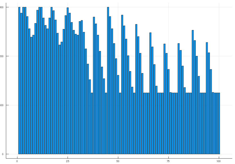
With this solution I obtained after even running it for 4 days straight on my machine only the deep local optimum just short of a bit more than 20$ from the global optimum.
I played with some setting of Gurobi next: See all
MIPFocus focus on finding better incumbents instead of focusing on the bound
Heuristics Spend more time on finding a new incumbent
Well I really wanted the optimal solution and others proved already that it is optimal so I don't have to. This all didn't work out as planned.
In the end I was glad that I still ranked 51/1620 and got my third silver medal.
Then shortly after the challenge people posted how they got there.
After the challenge
Some mentions first from the discussions forum that I found especially interesting:
By Gilles Vandewiele: Our journey towards the optimum
A long blog post from start to end
Including code and visualizations
By Bang Nguyen: My Optimal solution
Estimating the occupancies first (roughly) and then limit the change from these estimates to find the optimal solution. (Can't proof it's optimal)
By CPMP: John does California Odyssey (with code)
Several points on MIP, LP, local search
The 13th place (last gold medal ;) )
By Vlado Boza: Our trick
Very short and I will explain part of this in the following
By felixoneberlin: How to win Santa's Workshop Tour
His journey from the worst score to the optimal solution and being first in the challenge
So how to obtain the optimal solution given what we currently have. Actually there are only three small changes I did.
Set MIPFocus to 3 -> actually focus on the bound instead as this moves slowly
Reduce the number of possibilities (going away from proving optimality)
Add an extra variable for the occupancy on a single day
I think the first is simple. A bit more to the second point:
We can assume that we probably don't pay any family a helicopter ride because it is just super expensive so I've assumed that we don't pay more than 500$ per family by setting those x values to 0. That of course means that we can't prove optimality with this approach but don't worry we will later.
The third point is the most interesting I think and makes only sense if we roughly know how Gurobi works and I mean very very rough. Every MIP solver has this component or branch and bound which means that we solve as if every variable can be a floating point number and later we create a tree structure. If a variable x currently has a value 2.4 but should be integer we create two new models one where we add the constraint:
and one with:
\[ x \geq 3 \]This means that we remove the current solution but no real integer solution. Then we use some heuristics and cool tools to go down one of those paths (we might use the other one later). The key point is that with about 3 million binary variables we have a lot of variables to choose from but each step we only make a tiny choice. Therefore we can add a variable which doesn't represent new information but instead just helps with this branching. Meaning we use the new occupancy variable which is integer and has bounds 125 and 300. Then branching on such a variable cuts the tree in a half where on day 5 for example we have either \(\leq 200\) people or \(\geq 201\) people which is a bigger choice then saying we have exactly 200 people on day 89 and 214 on day 90 before christmas on the one hand or not on the other because fixing it to 0 still leaves sooo many options.
With these three changes I was able to find the optimal solution and proof it's optimal (given the constraint we don't pay more than 500$ per family) in about 44 hours with using some of my 69xxx solutions as a starting point.
Now after finding the optimal solution I was able to set it as my start point and then remove the 500$ per family constraint and run it again. Then after another 21 hours I (I mean Gurobi) was able to prove optimality of that solution.
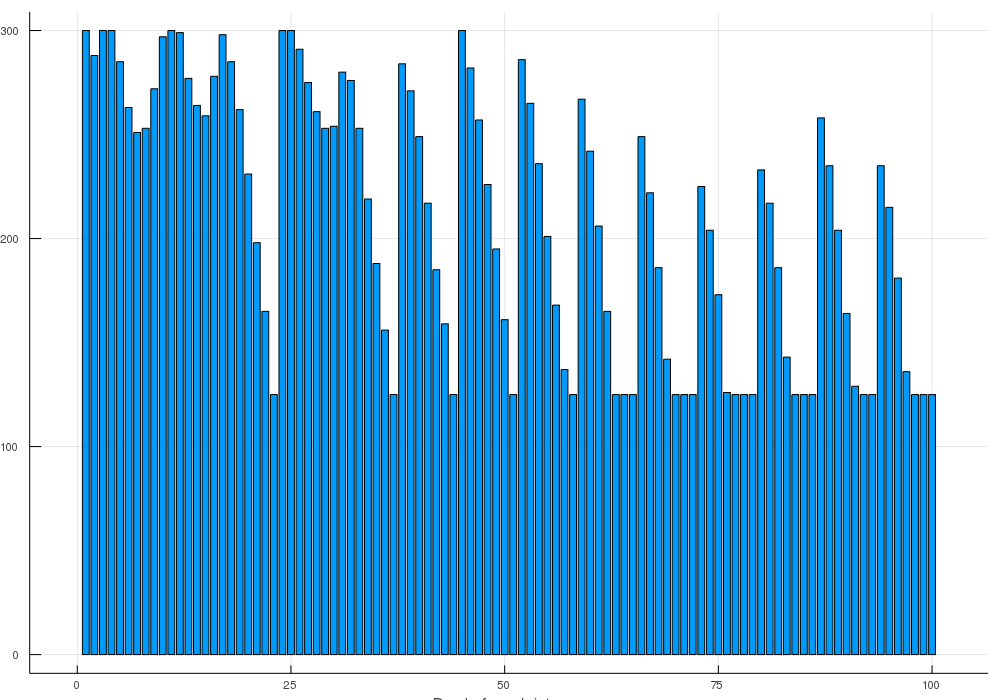
and you can see compared to the deep local minimum:
that we have one more dip down to 125.
I hope you enjoyed reading this final post and hopefully we will compete at the end of this year again.
Thanks for reading and special thanks to my five patrons!
List of patrons paying more than 2$ per month:
Site Wang
Gurvesh Sanghera
Currently I get 10$ per Month using Patreon and PayPal when I reach my next goal of 50$ per month I'll create a faster blog which will also have a better layout:
Code which I refer to on the side
Code diffs for changes
Easier navigation with Series like Simplex and Constraint Programming
instead of having X constraint programming posts on the home page
And more
If you have ideas => Please contact me!
For a donation of a single dollar per month you get early access to the posts. Try it out at the start of a month and if you don't enjoy it just cancel your subscription before pay day (end of month).
Any questions, comments or improvements? Please comment here and/or write me an e-mail o.kroeger@opensourc.es and for code feel free to open a PR/issue on GitHub ConstraintSolver.jl
I'll keep you updated on Twitter OpenSourcES as well as my more personal one: Twitter Wikunia_de
Want to be updated? Consider subscribing on Patreon for free
