Learning using a sigmoid neuron

In this blog entry you will learn how to teach your computer to learn something very simple for a start.

Last month I wrote a bit about perceptrons and sigmoid neurons. With this basic knowledge about the underlying structure machine learning makes use of, you are now well prepared to go a step further on your journey “Becoming a machine learning expert”. One of the things I hope you “saved in mind” is that sigmoid neurons are better to learn things, because they support non binary outputs. This is important to calculate an accurate deviation of our prediction.

Let's try to teach our computer to learn the logical functions "and" (\(\wedge\)) and "or" (\(\vee\)).

\(x_1\)	\(x_2\)	\(x_1 \vee x_2\)	\(x_1 \wedge x_2\)
0	0	0	0
0	1	1	0
1	0	1	0
1	1	1	1

We need a sigmoid neuron with only two inputs \(x_1,x_2\) and a single output for either \(x_1 \vee x_2\) or \(x_1 \wedge x_2\).

The machine should be able to learn both logical functions without changing the code. At the end we only want to change the input of our program, which includes both the input and the output of our sigmoid neuron. Therefore we need to build a general program to solve this problem. In this case the inputs will be the same for both functions, only the outputs differ.

The first step is to initialize our weights and bias. To make it easier, we will set them all to 0. Normally we would initialize them randomly, but it's easier to follow the steps when we set them to 0.

Our function to evaluate the output was defined as:

\(b := bias := -\text{threshold}\) \[ output = \sigma\big(\sum_i w_ix_i+b\big) = \sigma\big(\sum_i w_ix_i\big) \]

In the last equation we use that \(x_0=1\) and \(w_0 = b\).

\(\sigma(x)\) is the sigmoid function which is defined as:

\[ \sigma(x) = \frac{1}{1+e^{-x}} \]

Let's have a look at the first predicted output, where the real output is \(x_1 \vee x_2\):

\(x_1\)	\(x_2\)	real output	predicted output
0	0	0	0.5
0	1	1	0.5
1	0	1	0.5
1	1	1	0.5

To learn things we need to know how good our nidek is at the moment, so is the predicted output near the real one or is it completely wrong?

A really basic cost function would be:

\[ \begin{aligned} cost(real,pred) &= mean(real-pred) = \frac{1}{n}\sum_{i=1}^n (real_i-pred_i) \\ n &= \text{ number of outputs} \end{aligned} \]

Because real and pred are arrays, real-pred is an array as well, where real-pred is defined as the element-wise subtraction. Our cost function should be a single number, so we will take the mean value. There is a big problem with this basic cost function, which will be clear after looking at the first two predictions:

\(x_1\)	\(x_2\)	real output	predicted output
0	0	0	0.5
0	1	1	0.5

Here the cost will be 0, because \(mean(-0.5,0.5)=0\). A simple workaround is to use the root-mean-square:

\[ cost(real,pred) = \sqrt{mean((real-pred)^2)} = \sqrt{\frac{1}{n}\sum_{i=1}^n (real_i-pred_i)^2} \]

Now the total costs are 0.5 which makes sense, because every predicted output has a difference of 0.5 to the real output. We will try to minimize this cost to achieve our goal to predict the logical "or" function precisely. Let's make a quick visualization where we change the weights and see how the cost function changes.

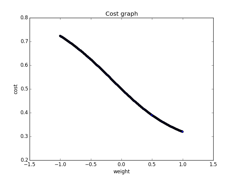
To make the graph 2D I set the bias to 0 and the weight is now the weight for both inputs. Which makes sense in this logical case, but normally it isn't true. We can see that higher weights (near 1) minimize the output. But 'we don''t want to draw the weights and have a look and set the weights by hand and we also don't want to try a lot of weights and choose the best. We want a method to find the optimum.

We can imagine that the graph is a landscape (yes, here a 2D one), and we lay down a ball where the weights are set to 0. Now the ball rolls to the minimum and our goal is to program this behavior. We don't need to build a real physics engine for that, which makes everything a lot easier.

I hope you all have/had some analysis in school or university, because we need some math here. We will use the gradient to minimize the costs. This technique is called gradient descent. If the gradient is negative, the ball would roll in the right direction, so we will choose a higher weight to minimize the cost.

The derivative of the cost function is:

\[ \frac{\delta cost}{\delta w_j} = \frac{2}{n} \sum_{i=1}^n x_j (pred_i-real_i) \]

Here \(w_j\) are the weights (\(w_0\) is the bias), \(j \in \{0,1,2\}\).

Normally the \(\frac{2}{n}\) is a \(\frac{1}{n}\), which will be true, if we set the cost function to:

\[ cost(real,pred) = \sqrt{\frac{1}{2n}\sum_{i=1}^n (real_i-pred_i)^2} \]

so using the half of the mean. Now the gradient, which is more important for the program, is:

\[ \frac{\delta cost}{\delta w_j} = \frac{1}{n} \sum_{i=1}^n x_j (pred_i-real_i) \]

We want to use this function, because it's the common definition.

Remember: \(x_0\) is defined as \(1\).

To compute the new weights, we need to subtract the gradient from the last weights.

\[ w_{j_{\text{new}}} = w_{j_{\text{old}}}-\alpha \frac{\delta cost}{\delta w_j} \]

Here alpha is the so called learning rate, kind of the speed of the ball. If the speed is too high, the ball can roll upwards, but if the learning rate is too small, we can wait a long time until we find good weights, so we need to find a learning rate in the middle.

You can always try several learning rates and visualize the cost function in some way, and if it's not falling down, you should lower it, and if it's falling down too slow, you can try a higher learning rate.

Let's try to really code our first learning program.

I always use Python and because of some libs I am unfortunately using v2.7. The best lib, which I use in every program is numpy:

import numpy as np

First of all we need to define our functions to predict the outcome:

def sigmoid(x):
    return 1.0/(1+np.exp(-x))

"""
    Predicts the outcome for the input x and the weights w
    x_0 is 1 and w_0 is the bias
"""
def predict(x,w):
    return sigmoid(np.sum([w[p]*x[p] for p in range(len(x))]))

"""
    initialize the weights w, inputs x and outputs y
    here the outputs are the outputs for x[1] or x[2]
"""
w = np.array([0,0,0])
# the first value in each subarray is the weight of the bias input,
# which is always set to 1
x = np.array([[1,0,0],[1,0,1],[1,1,0],[1,1,1]])
y = np.array([0,1,1,1])

The prediction is the same as defined at the very beginning.

\[ output = \sigma\big(\sum_i w_ix_i\big) \]

To see how good our program is, we will define our cost function:

"""
    Determine the cost of the prediction (pred)
"""
def cost(real,pred):
    return np.sqrt(1.0/2*np.mean(np.power(real-pred,2)))

\[ cost(real,pred) = \sqrt{\frac{1}{2n}\sum_{i=1}^n (real_i-pred_i)^2} \]

But now we really want to learn ;) Let's define the gradient function:

"""
    get the gradient for the inputs x,weights w and the outputs y
"""
def gradient(x,w,y):
    # create an empty gradient array which has the same length as the array of weights
    grads = np.empty((len(w)))
    # compute the gradient for each weight
    for j in range(len(w)):
        grads[j] = np.mean(np.sum([x[i,j]*(predict(x[i],w)-y[i]) for i in range(len(x))]))
    return grads

"""
    get the new weights based on the old ones w, learning rate a and the gradients
"""
def getWeights(w,a,grads):
    return w-a*grads

Let's make use of all these functions to learn the "or"-function:

"""
    Create a new array (prediction) which afterwards holds the prediction for the inputs x.
"""
prediction = np.empty((len(x)))
for i in range(len(x)):
    # calculate the prediction for each input (keep the weights unchanged)
    prediction[i] = predict(x[i],w)
    print("prediction for: ",x[i]," is ",prediction[i])

# get the costs of the prediction
print("Cost: ")
print(cost(y,prediction))
# calculate the gradients
print("Grads: ")
grads = gradient(x,w,y)
print(grads)
# get the new weights using a learning rate of 0.3
print("New Weights: ")
a = 0.3
print(getWeights(w,a,grads))

The output is the following:

('prediction for: ', array([1, 0, 0]), ' is ', 0.5)
('prediction for: ', array([1, 0, 1]), ' is ', 0.5)
('prediction for: ', array([1, 1, 0]), ' is ', 0.5)
('prediction for: ', array([1, 1, 1]), ' is ', 0.5)
Cost:
0.353553390593
Grads:
[-1. -1. -1.]
New Weights:
[ 0.3  0.3  0.3]

First, we get the prediction for each input, which is 0.5, as expected. The cost looks a bit different, because we used the root-half mean-square error here. The gradient means, that the graph falls and we should use higher weights. The learning rate of 0.3 is just a random guess.

Let's make some more learning steps. We just need to define the new weights as w (next to last line) and make a for loop:

a = 0.3
for c in range(50):
    prediction = np.empty((len(x)))
    for i in range(len(x)):
        # calculate the prediction for each input (keep the weights unchanged)
        prediction[i] = predict(x[i],w)
        print("prediction for: ",x[i]," is ",prediction[i])

    # get the costs of the prediction
    print("Cost: ")
    print(cost(y,prediction))
    # calculate the gradients
    print("Grads: ")
    grads = gradient(x,w,y)
    print(grads)
    # get the new weights using a learning rate of 0.3
    print("New Weights: ")
    w = getWeights(w,a,grads)
    print(w)

The last output (after 50 learning steps):

('prediction for: ', array([1, 0, 0]), ' is ', 0.27814770422749474)
('prediction for: ', array([1, 0, 1]), ' is ', 0.8956866585480121)
('prediction for: ', array([1, 1, 0]), ' is ', 0.8956866585480121)
('prediction for: ', array([1, 1, 1]), ' is ', 0.99480086855592609)
Cost:
0.11133043314
Grads:
[ 0.06432189 -0.10951247 -0.10951247]
New Weights:
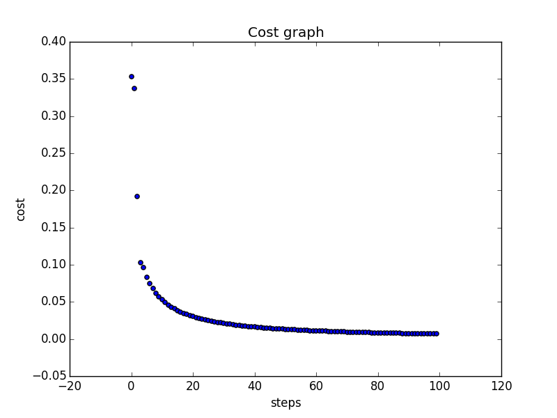
[-0.97296483  3.13671337  3.13671337]

That's quite good, our program "thinks" to 99%, that \(1 \vee 1\) is 1 and \(0 \vee 0\) is 0 with a probability of around 72%. That isn't too bad. We have to keep in mind, that it's not a common case to predict functions that are well defined, like that logic function. Normally we want to predict things where we don't know how to create a formula. I totally love visualizations so let's visualize the costs of our prediction, which we compute using the costs function.

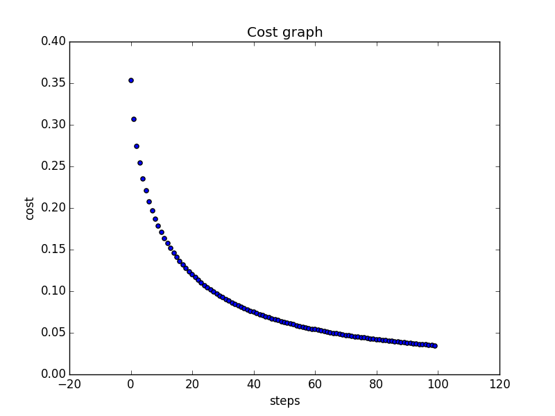
It's a bit slow, right? Let's try a higher learning rate, like 3.

And yes this one looks much better. The output for the prediction is:

('prediction for: ', array([1, 0, 0]), ' is ', 0.01662680782493511)
('prediction for: ', array([1, 0, 1]), ' is ', 0.9933572664074547)
('prediction for: ', array([1, 1, 0]), ' is ', 0.9933572664074547)
('prediction for: ', array([1, 1, 1]), ' is ', 0.99999924391101913)
Cost:
0.00675187527823
Grads:
[ 0.00334058 -0.00664349 -0.00664349]
New Weights:
[-4.08999413  9.10746966  9.10746966]

You've learned how to teach a computer to learn the most simple stuff!

Is it possible to change the outputs y to:

y = np.array([0,0,0,1])

to learn the "and"-function, without changing any code?

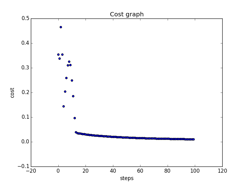
Yes it is, but here you can see, that it isn't always a good idea to use a high learning rate. The cost isn't falling down all the time. Using a learning rate of 1 looks smoother, which is better, because we are decreasing the costs in each step.

You can always download the code I used here via Github.

In the next entries you'll learn how to program some more awesome things. One interesting thing is to predicte how likely it is that a person with defined characteristics survied the Titanic disaster. For that special case we know the answer but it might be interesting for future disasters. There is a Kaggle challenge where you can download the Titanic datasets.

Helpful links

Andrew Ng made an awesome online course about machine learning, where you get more theoretical insights: Machine Learning at Coursera by Andrew Ng

A neat comic by xkcd about this topic:

Want to be updated? Consider subscribing on Patreon for free