Master thesis: Minimum degree ordering
Creation date: 2021-07-09

I finally managed to finalize my master thesis and submitted it a couple of days ago. In this post I would like to tell you what it is about and try to keep it short 😉
Some basic understanding of linear algebra and graph theory will hopefully get you quite far in this post. I'll not go into discussing results and future ideas in this post but rather explain the problem and a solution. The thesis was built on top of a variety of already existing research. Which should be obvious 😄
In this post I want to give a rough explanation as more of an introduction into the problem and the idea of an algorithm that solves it. Later posts cover how to make the basic algorithm fast and maybe another one on how to further apply different ideas to make it even faster.
I point to learning resources and related work at the end of this post.
Let's get started:
Short Description of the Problem
In a variety of different scientific fields one encounters systems of linear equations like:
\[ Ax = b \]with \(A\) being a matrix and \(x\) and \(b\) vectors, \(A\) and \(b\) are given and we want to find the \(x\). Yeah as always in mathematics... They only care about what \(x\) is.
Often that matrix \(A\) is sparse which roughly means that it has only a few non-zero elements or rather most elements are 0. Let's go one step deeper into specialization by only having a look at symmetric matrices 😉 Those are matrices which are symmetric regarding the upper left to lower right diagonal.
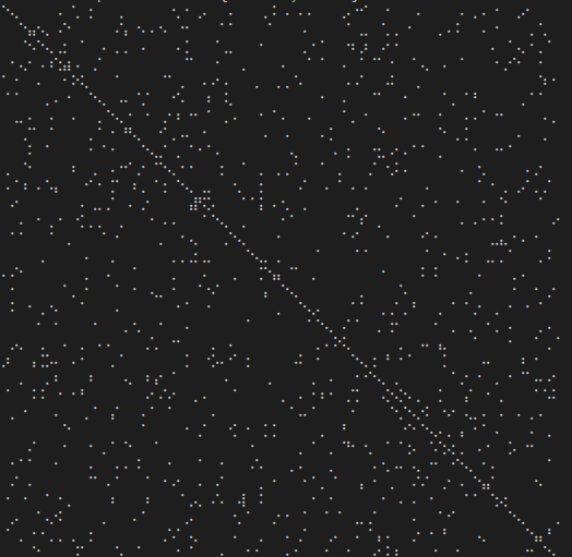
Here you can see the sparsity pattern of a random 1000x1000 matrix + diagonal entries which has only 2112 non-zero elements. The non-zero elements are represented by a white dot and black indicates zeros. You'll see a smaller example later.
Now you might know that solving linear systems normally involves decomposing the matrix \(A\) into matrices which have a defined structure which make it easier to solve the system.
As an example
\[ \begin{pmatrix} 1 & 7 \\ 7 & 9 \end{pmatrix} \begin{pmatrix} x_1 \\ x_2 \end{pmatrix} = \begin{pmatrix} 3 \\ 5 \end{pmatrix} \]Here we have a dense matrix (with actually no zeros) but it isn't obvious what \(x_1\) and \(x_2\) are.
\[ \begin{pmatrix} 1 & 0 \\ 7 & 1 \end{pmatrix} \begin{pmatrix} y_1 \\ y_2 \end{pmatrix} = \begin{pmatrix} 3 \\ 5 \end{pmatrix} \]Solving this on the other hand is quite straightforward as we can see that \(1 y_1 + 0 y_2 = 3\) implies that \(y_1 = 3\). We can use that to have \(3\cdot 7 + y_2 = 5\) and get \(y_2 = 5-21=-16\).
\[ \begin{pmatrix} 1 & 7 \\ 0 & -40 \end{pmatrix} \begin{pmatrix} x_1 \\ x_2 \end{pmatrix} = \begin{pmatrix} 3 \\ -16 \end{pmatrix} \]Can be solved in a similar way to get \(x_2 = 0.4\) and \(x_1 + 0.4 \cdot 7 = 3\) evaluates to \(x_1 = 0.2\).
Okay great (2) is hard to solve because one can't easily get one variable as no coefficient in the matrix is zero. Equations (3, 4) however are easy to solve because one coefficient is zero and the result can be easily read. But how does that solve the problem we have in the first place?
Well actually if we compute
\[ \begin{pmatrix} 1 & 7 \\ 7 & 9 \end{pmatrix} \begin{pmatrix} 0.2 \\ 0.4 \end{pmatrix} = \begin{pmatrix} 3 \\ 5 \end{pmatrix} \]We see that \((0.2, 0.4)^\top\) is a solution to the original problem. The question now is therefore: How to get those easy matrices?
Those matrices can be obtained by decomposing the matrix which basically means we solve \(A = LU\) where \(L\) is a lower triangular matrix (has only non-zero values in the lower left) and \(U\) being an upper triangular matrix where the non-zero values are on the upper right.
There are different kinds of decompositions like the Cholesky decomposition or the one mentioned above which is simply called LU decomposition.
Everything is faster and easier to solve now but we introduce a problem which I tackled in my thesis.
It's often the case that decomposing the matrix creates additional non-zero elements in both \(L\) and \(U\). Due to the fact that we deal with sparse matrices we only want to save the values and positions of those non-zero elements.
As an example if we have a 1000x1000 matrix with only 2500 non-zero elements we can either save 1 million (1000 x 1000) elements or about 3*2500 = 7500 by saving both the row, column positions as well as the value. One can further reduce this, but as you can see already: It saves a lot of memory by storing only the non-zero values explicitly.
Now if we use the decomposition and create a lot of new non-zero elements we might increase the memory consumption so much that it's impossible to solve the system. In some cases the decomposition creates two completely filled lower and upper triangular matrices in which case we would need to store 3 million entries or convert it into a dense matrix but still would need to store 1 million values.
One interesting fact that we can use is that we can permute the matrix rows and columns and do the same for \(x\) and \(b\) and still get the right solution.
As an example
\[ \begin{pmatrix} 9 & 7 \\ 7 & 1 \end{pmatrix} \begin{pmatrix} 0.4 \\ 0.2 \end{pmatrix} = \begin{pmatrix} 5 \\ 3 \end{pmatrix} \]is just a permuted version of the equation we had before.
Graph Theory?
Well I said at the very beginning that this has something to do with graph theory, right? Let's have a look at a symmetric matrix again which is in between of the two sizes we had before. Let's say a \(5 \times 5\) matrix. As in the sparsity pattern case we don't care about the values inside the matrix but use a one for explanation here. We normally only care where the non zeros are. You'll understand why in a minute:
\[ \begin{pmatrix} 1 & 1 & 1 & 1 & 1 \\ 1 & 1 \\ 1 & & 1 \\ 1 & & & 1 \\ 1 & & & & 1 \end{pmatrix} \]If we want to create a upper triangular matrix we multiply a row by a scalar (a number) and add rows together. The lower triangular matrix is basically the counter part of this where we save how we did this to be able to get the starting matrix multiplication. That part however isn't relevant here but please feel free to dive deeper for example with Gaussian elimination.
We focus on the upper triangular matrix here so we want to have zeros in the lower left part. This can be done by having \(r_2 = r_2 - r_1\) where \(r_j\) is the \(j\)-th row. We can actually do this for all rows \(2\) to \(5\) to create this:
\[ \begin{pmatrix} 1 & 1 & 1 & 1 & 1 \\ & & -1 & -1 & -1 \\ & -1 & & -1 & -1\\ & -1 & -1 & & - 1 \\ & -1 & -1& -1 & \end{pmatrix} \]Now you can see that we created a lot of non-zero entries while achieving our goal of creating zeros in the first column (besides the first row which is part of the diagonal and can therefore have a non-zero value). This is only the first step of creating the upper triangular matrix but it already shows the problem. 😉
The matrix in (7) was actually quite sparse but the decomposition is a completely dense matrix. We applied only one step of Gaussian elimination but it will not get sparser after more steps.
Let's do some graph theory finally! 😉
We can represent the symmetric matrix (7) as graph with 5 nodes (as it's a \(5 \times 5\) matrix).
Whenever a row column pair has a non-zero value as (1,2), (1,3), (1,4) & (1,5) in (7) we connect the corresponding nodes with an edge. You might wonder why we change the representation of the problem. This is the case because we will see a common structure in graph theory appear when we do our decomposition steps. We already know theory about those graphs that we can apply here and another thing is that the graph representation removes the notation of the specific values in the matrix. We only care about zero or non-zero which here gets represented as an edge.
Now when we apply one elimination step we only have to change rows which have a non-zero value at the position where we want to create a zero.
As an example
\[ \begin{pmatrix} 1 & 0 & 1 & 1 & 1 \\ 0 & 1 \\ 1 & & 1 \\ 1 & & & 1 \\ 1 & & & & 1 \end{pmatrix} \]in this case we don't need to change row 2 as it already has a zero as its first entry.
Now in the graph this means we have to check the edges of the node we want to eliminate. This is due to the fact those connections determine the new edges we need to create. In our case we want to eliminate node 1 (row and column 1) to reduce the size of the matrix (number of rows/columns) by 1.
If two nodes are connected we have to perform a calculation. The thing of interest is now how do we represent the change in the matrix due to this calculation in the graph? One can see that in (9) we wouldn't need to create non-zero values in the second row in our first elimination step as we don't touch that row. However we would fill the rest of the upper triangular matrix.
When we focus on row 3 for a second we compute something like \(r_3' = r_3 + x \cdot r_1\). As row 1 has non-zero values at position 4 and 5 we might introduce non-zero values in row 3 at those positions. So we always connect the nodes together which were previously neighbors of current elimination node.
In the graph representation this can be achieved by forming a clique of the previous neighbors of the node we want to eliminate and removing the edges to the previous connected neighbors. I'll formally define a clique in a second but for now you can see it as a subset of nodes which are all directly connected to each other like a clique in real life. 😄
You can see that the nodes 2 to 5 form a clique now.
Fundamentals of Graph Theory
Just a few points of what a graph is and what a clique is and so on 😉 . If you have basic knowledge of graph theory you can skip most of it but might come back when I have a different notation than you.
We name graphs as \(G=(V,E)\) where \(V\) is a set of nodes and \(E\) is a set of edges \(\{u,v\}\) where \(u, v \in V\). Now to define a clique we need the notion of a complete graph and an induced subgraph. A complete graph \(K\) is a graph in which every node is connected (adjacent) to every other node. A subgraph \(G[A] := (A, E(A))\) is the induced subgraph of nodes \(A\) with \(E(A) := \{\{v,w\} \in E \mid v,w \in A \}\).
Let's also define \(N(v) := \{w \in V \mid \{v,w\} \in E\}\) which just defines the neighbors of \(V\).
That should hopefully be enough to understand the idea of the algorithm.
An Idea for an Algorithm
Now we have seen that we always need to form a clique of neighboring nodes when we eliminate one node from our graph. When we eliminate \(v\) we add at most \(\|N(v)\| \cdot (\|N(v)\| - 1) / 2\) edges.
Which increases quadratically by the number of neighbors. Now we want to keep the decomposed triangular matrices as sparse as possible. That means we want to reduce the number of edges that we want to add. The idea for that is rather simple: We just pick the node next that has minimum degree (the minimum number of neighbors).
This technique is called: Minimum degree ordering
The post is already rather long so I don't want to explain how it's implemented in this post but maybe you can already think about the following questions:
What is the run time of a naive implementation of this algorithm?
Which parts take the most time to compute
Ideas on how to reduce the running time
All of this will be tackled in the next post which should be available by next week. If you don't want to miss that post as well as others which are mostly about Julia graph theory, constraint programming and visualizations please consider subscribing to my free email newsletter:
Free Patreon newsletterOther Algorithms that solve the same Problem
The above mentioned algorithm is only a heuristic, so it does not give a permutation with a minimum number of fill-in edges. Computing those kinds of permutations however is an NP-hard problem Yannakis (1981).
Most if not all interesting problems in computer science are those where there is no fast algorithm which gives the optimal solution. In those areas many different ideas come together to find better and faster heuristics. This area of research is no different.
Before we checkout different algorithms I would like to point to the paper George & Liu (1989) about the evolution of the above described minimum degree ordering algorithm if interested.
Therefore there are at least two different algorithm ideas to solve this minimum node ordering problem. Nested dissection is an approach in which a graph is partitioned into smaller graphs recursively and then those smaller graphs are ordered independently. The sub orderings are then simply combined together. That approach is much faster than minimum degree ordering but sometimes provides worse results as the orderings are just concatenated together George & Liu (1978). This algorithm also often works with so called data reduction rules which I'll explain in the next post. You can however read about them already if interested Ost et al. (2021).
Another approach is called Approximate minimum degree ordering in which case only an approximate degree of the nodes is used. Those approximations are faster to compute which provides a benefit over the exact minimum degree ordering. However depending on the approximations they can provide worse results as well Amestoy et al. (1996).
In both cases the results depend quite a lot on the graph itself. Finding out for which instances each of the algorithms performs best is still open for research 😉
Bibliography
Yannakis: Computing the Minimum Fill-In is NP-Complete
George & Liu: The Evolution of the Minimum Degree Ordering Algorithm
George & Liu: An Automatic Nested Dissection Algorithm for Irregular Finite Element Problems
Ost et al.: Engineering Data Reduction for Nested Dissection
Amestoy et al.: An Approximate Minimum Degree Ordering Algorithm
Thanks everyone for reading. Hope you enjoyed it and learned something. If you're repeatably happy on this blog please consider subscribing 😉
Thanks to my 13 patrons!
Special special thanks to my >4$ patrons. The ones I thought couldn't be found 😄
Anonymous
Kangpyo
Gurvesh Sanghera
Szymon Bęczkowski
Colin Phillips
Jérémie Knuesel
For a donation of a single dollar per month you get early access to these posts. Your support will increase the time I can spend on working on this blog.
There is also a special tier if you want to get some help for your own project. You can checkout my mentoring post if you're interested in that and feel free to write me an E-mail if you have questions: o.kroeger <at> opensourc.es
I'll keep you updated on Twitter OpenSourcES.
Want to be updated? Consider subscribing on Patreon for free
