TSP: Greedy approach and using a 1-Tree

About four years ago I published a blog post about solving the traveling salesman problem in Julia. Feel free to read the approach using mixed integer programming there. It also sparked the idea for the TravelingSalesmanExact.jl package by one of my readers.

Introduction to the TSP

You probably know already what the Traveling Salesman Problem (TSP) is, but maybe you are new to mathematical optimization and I'm glad to have you on this blog 😉 Ever wondered how to plan a route to different shopping centers in your city that you want to visit from home and then return back home? You are probably interested in the shortest total length for this and this is the traveling salesman problem 😄 It can be applied to various kinds of problems like to someone who wants to sell the newest phone by walking from door to door in a city. You know back in those days before the internet arrived and you don't talk to traveling salesman anymore... Guess what though: How does a company like Amazon plan their route to bring you the newest smartphone? They use some kind of traveling salesman approach. However, often it gets more complicated as the shopping centers have different opening ours or you probably buy something bigger in one of them and don't want to carry it over to the others.

Well, we have to solve the basics before we can tackle harder ones. Therefore, we continue with the general TSP in this series. I'll also focus only on the symmetric case, which means traveling from \(A\) to \(B\) has the same cost as traveling from \(B\) to \(A\).

The old approach

The general approach in my first post was to find the shortest tour by always minimizing the cost of the chosen edges under the following constraints:

• Each city needs to be visited a single time (-> means it needs to have exactly one incoming and exactly one outgoing edge)

• A city can't have itself as a neighbor (so we want actual edges not those of zero cost)

What normally happens in that case though is that one gets a lot cycles often of length two as you can see below.

Then the next steps were a repetition of finding cycles and disallowing them. After disallowing all 1-1 cycles this was the result:

This was repeated until there was only the big cycle that we want to obtain.

Preface of this series

I wanted to have another look at the problem and try out different approaches and blog about them in a similar fashion as I do with my constraint solver series. If you are interested in following my trial and error approach please consider subscribing to my email list.

Free Patreon newsletter

In this post I want to build two different things which will be the basic building blocks for a while. The above approach is a way to always minimize the cost as much as possible but never have an actual tour until the very last step. This means we always have a lower bound to the actual cost. This post will explain a different kind of lower bound using minimum spanning trees. The other part will be a greedy approach which always picks the next edge that minimizes the connection to another city.

In the following posts I'll then try to provide either a better heuristic which finds actual tours or trying to find better lower bounds. The goal is to squeeze the range of the length of the best solution from both sides. The general approach will be to fix some edges then or disallow some in a branch and bound procedure to obtain the shortest tour.

TSP Benchmark

It is always nice to see how long it takes for a current approach to solve the problem. Then we have a baseline and know whether our approach is slower, faster or about the same. Here I should probably note that there are way faster approaches than the one that is currently implemented in the TravelingSalesmanExact.jl package. Which means we have chances to beat the current approach 😄

using TravelingSalesmanExact, GLPK

points = simple_parse_tsp("data/bier127.tsp")
set_default_optimizer!(GLPK.Optimizer)
# compile run
get_optimal_tour(points; verbose=false)

@time get_optimal_tour(points; verbose=false)

I've downloaded the cities from zib.de. You can see more problems on their overview site.

Currently it takes about 8.2s on my machine on this 127 point problem. The tour length is: 118293.52381566973

For future posts I'll test out a set of different problems to get a good overview but as long as we don't have a competitor we can just keep it like this for now.

Greedy approach

Let us start with the simpler upper bound approach. We create the cost matrix first and then start at the first point and connect it to the nearest neighbor. Then we go from that neighbor and connect it to the nearest one which we haven't in our tour yet.

const TSP = TravelingSalesmanExact
N = length(points)
cost = [TSP.euclidean_distance(cities[i], cities[j]) for i = 1:N, j = 1:N]

The euclidean_distance function is part of the TravelingSalesman package.

Now to the greedy approach:

function greedy(points, cost)
    N = length(points)
    visited = Set{Int}(1)
    tour = Int[1]
    last_city = 1
    while length(tour) < N
        last_city = argmin(j->j in visited ? Inf : cost[j, last_city], 1:N)
        push!(visited, last_city)
        push!(tour, last_city)
    end
    return tour
end

We have a set of all visited points to disallow adding them more than once to the tour. Then we set the distances to those unwanted points to infinity which avoids picking them with argmin.

using Luxor

function get_luxor_coords(points; w = 600,h = 600)
    # padding
    w -= 20
    h -= 20
    minx, maxx = extrema(p->p[1],points)
    miny, maxy = extrema(p->p[2],points)
    w, h = 580, 580
    pts = [Point((p[1]-minx) / (maxx-minx) * w - w/2, (p[2]-miny) / (maxy-miny) * h - h/2) for p in points]
    return pts
end

function draw_tour(points, tour)
    coords = get_luxor_coords(points)
    @png begin
        sethue("black")
        for i in 1:length(tour)-1
            src = tour[i]
            dst = tour[i+1]
            line(coords[src], coords[dst], :stroke)
        end
        line(coords[tour[end]], coords[tour[1]], :stroke)

        sethue("blue")
        circle.(coords, 3, :fill)
    end 600 600 "tour.png"
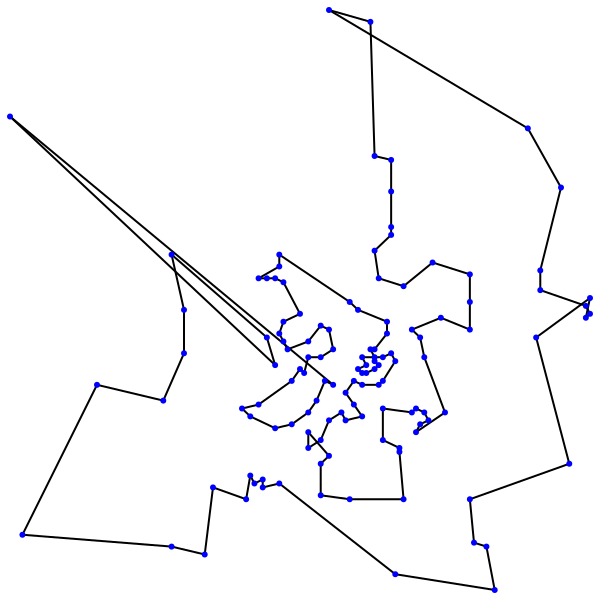
end

With the above functions we can plot our tour using Luxor . We first make sure that all points fit into the 600x600 canvas with the get_luxor_coords function. In the draw_tour function we draw a line for each edge and a circle for each point. We can see that some parts already look reasonably well but in some others we have very long edges. Which makes sense as at later stages a lot of points are already on the tour and we have to reach far to connect yet another one to the tour.

Next up we need a function to get the cost of our tour.

function get_tour_cost(tour, cost_mat)
    cost = 0.0
    for i in 1:length(tour)-1
        src = tour[i]
        dst = tour[i+1]
        cost += cost_mat[src,dst]
    end
    cost += cost_mat[tour[end],tour[1]]
    return cost
end

For our greedy tour we get a length of ~135751.77 which is about 15% longer than the optimal tour. There are definitely some straightforward ways to improve that tour by doing some swapping as crossing lines are always bad.

Lower bound using minimum spanning tree

However, we don't want to dive too deep in this first post as I don't have anything for the next posts then 😄 Well actually there are some many people who worked on heuristics that I would probably never stop writing when I want to understand, implement and blog about all of them. Nevertheless, let's start with a lower bound now. One thing that the previous method of TravelingSalesmanExact.jl didn't do is having a connection of all the points. We had basically had several traveling salesman tours for smaller problems.

This time I want to not have tours but have a connected structure such that we can reach all the cities. I should probably mention at various points of this series that most if not all of these ideas that I have are actually not mine. A lot of researchers spent years on this problem and I just try something out and read about their approaches. This connected structure approach is by Held & Karp. which I read about in this fantastic book: The Traveling Salesman Problem: A Computational Study.

Finding the shortest connected structure is the problem of finding a minimum spanning tree. It is a pretty easy problem to solve and is kind of similar to our greedy TSP approach from above. We pick a random start node, sort all the possible edges from there by length and pick the shortest one. Then we pick the one shortest edge which connects a new vertex with the already existing structure until we have connected all the nodes.

This is called Prim's algorithm. Fortunately it is already implemented in Graphs . All we have to do is install it ] add Graphs and use it using Graphs 😄

using Graphs

function get_tree_cost(edges, cost)
    tour_cost = 0.0
    for edge in edges
        tour_cost += cost[edge.src, edge.dst] 
    end
    return tour_cost
end

function get_1tree(cost)
    tree = prim_mst(complete_graph(size(cost,1)), cost)
    tree_cost = get_tree_cost(tree, cost)
    return tree, tree_cost
end

I've named the function get_1tree here even though it is just a standard minimum spanning tree (MST) for now. This will be updated next 😉 prim_mst returns a vector of edges which we can easily loop over to get the cost of this tree.

Let's draw the solution of the MST:

function draw_tree(points, tree)
    coords = get_luxor_coords(points)
    @png begin
        sethue("black")
        for e in tree
            line(coords[e.src], coords[e.dst], :stroke)
        end

        sethue("blue")
        circle.(coords, 3, :fill)
    end 600 600 "tree.png"
end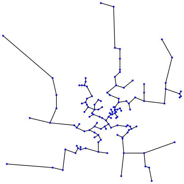

This tree has a cost of ~94718 which is roughly 20% lower than that of the optimal tour. Which means we currently have a relatively big gap between our lower bound and our upper bound. However we can do some more regarding the lower bound in this post.

Hope you still have time 😉

1-Tree and node weights

You can see above that we have a proper tree, which means we have no cycles. With the other implementation of finding a tour we started with many cycles and eliminated them until we only had one. This time we don't have any cycle but want one. We can pick one vertex and connect it to its two nearest neighbors and for all vertices excluding the one we picked we can call the MST function. Depending on which vertex we pick this can make some difference but it doesn't feel worth it to try out all of them to pick the best. At least when we have some much bigger idea first.

function get_1tree(cost)
    N = size(cities, 1)
    # we pick the last vertex as our start vertex to easily compute the MST for the first N-1
    tree = prim_mst(complete_graph(N-1), cost)
    mst_cost = get_tree_cost(tree, cost)

    # extra cost for the two edges from the last city to the two nearest neighbors
    nearest_neighbors = partialsortperm(cost[:,N], 1:3)
    n_actual_neighbors = 0
    extra_costs = 0.0
    for neighbor in nearest_neighbors
        n_actual_neighbors == 2 && break
        if neighbor != N
            n_actual_neighbors += 1
            push!(tree, Edge(N, neighbor))
            extra_costs += cost[neighbor, N]
        end
    end

    lb = mst_cost + extra_costs

    return tree, lb
end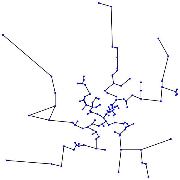

Here we can see on the left side that we have one cycle now.

One idea is now to try forcing the tree into a single cycle. Which means every node which has a single edge should gain another one while nodes which have three or more edges should loose those extra edges. We still want to have a 1-tree structure though. As we want that it remains a lower bound.

It is relatively straightforward to see that we can change the cost of the edges to \(c_{uv} = c_{uv} - c_{u} - c_{v}\) so every node gets an associated weight and when it's a positive weight we decrease all the edges around it by a certain amount and if it has a negative weight we increase the cost of the edges.

This will change the MST but it does not change the fact that it is a lower bound of the TSP as long as we later add \(2 \sum_{v \in V} c_v\) to the cost of the MST. It makes sense to do these changes of node weights a couple of times. We assign a positive weight on a node if it only has one incident edge and a negative weight if it has a degree of more than 2.

Below you can see a function which runs those steps num_of_runs times and my update formula here depends on the maximum cost in the cost matrix. I haven't figured out yet how to determine by how much it should update the node weights which I call benefit_factor.

function get_optimized_1tree(cost; num_of_runs=10)
    N = size(cost, 1)
    tree, lb = get_1tree(cost)
    degrees = zeros(Int, N)
    point_benefit = zeros(Float64, N)
    extra_cost = 0.0
    max_cost = maximum(cost)

    benefit_factor = max_cost/N
    for _ in 1:num_of_runs
        degrees .= 0
        point_benefit .= 0.0
        for edge in tree
            degrees[edge.src] += 1
            degrees[edge.dst] += 1
        end
        for i in 1:N
            point_benefit[i] = benefit_factor*(2-degrees[i])
           
            cost[i, :] .-= point_benefit[i]
            cost[:, i] .-= point_benefit[i]
        end
        extra_cost = 2*sum(point_benefit)
        tree, lb = get_1tree(cost)
        benefit_factor *= 0.9
    end

    return tree, lb+extra_cost 
end

This results in the following 1-tree:

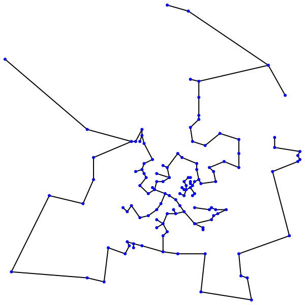
With this we obtain a lower bound of ~113139 which brings us to nearly 96% of the optimal tour. It also only takes about 2.5ms to compute this lower bound. This means we can do quite some more stuff before we reach the 8s from the current approach.

Next up

Well currently we have two approaches one for a lower bound and one for an upper bound but how to we bring them together? With the lower bound we don't really have a tour yet and our current upper bound isn't that great yet. In the long run we want to improve on both sides as much as possible. A reasonable next step however is probably to implement a branch and bound algorithm for this task.

In that we would start with a root node which has the information about the lower and the upper bound which we calculated today. Then we make decisions of the form: What happens to those bounds if we include this edge on the one hand or disallow it on the other hand? In each step of the lower bound calculation we also need to check whether it's already a tour or just a 1-tree.

This is my idea for the next post. In the next post I introduce a general branch and bound framework Bonobo . Read about it here.

Please let me know your thoughts via email or via twitter. See the links below.

As always: Thanks for reading and see you soon (don't forget to subscribe to the newsletter 😉)

Special thanks to my 12 patrons!

Special special thanks to my >4$ patrons. The ones I thought couldn't be found 😄

• Anonymous

• Kangpyo

• Gurvesh Sanghera

• Szymon Bęczkowski

• Håkan Kjellerstrand

• Colin Phillips

• Jérémie Knuesel

For a donation of a single dollar per month you get early access to these posts. Your support will increase the time I can spend on working on this blog.

There is also a special tier if you want to get some help for your own project. You can checkout my mentoring post if you're interested in that and feel free to write me an E-mail if you have questions: o.kroeger <at> opensourc.es

I'll keep you updated on Twitter opensourcesblog.

Want to be updated? Consider subscribing on Patreon for free