TSPSolver.jl: 2-opt

In the last post I've integrated Bonobo into my TSPSolver project and was able solve the first TSP instance. There we noticed that the current version is about 10x slower than the already existing package TravelingSalesmanExact.jl.

With the extras you'll read in this post the gap will be closed for that particular instance but will still be slower in a lot of our instances.

Improving the branching part

Last time we simply branched on the longest edge whether it is in the current tour or not. I reckoned it will be more reasonable to branch on a long edge which is part of the lower bound 1-tree but not part of the tour we found in that branch.

There are of course way more interesting things we need to do with the branching part. One such thing that might not be super helpful for TSP but will be for various other problems that Bonobo can be used for is strong branching. It's the default branching strategy for Juniper due to its effectiveness there.

Finding a better tour

In the last post I've argued that working on the problem of finding better upper bounds is valuable. The first tour we found for the berlin52.tsp instance was the following.

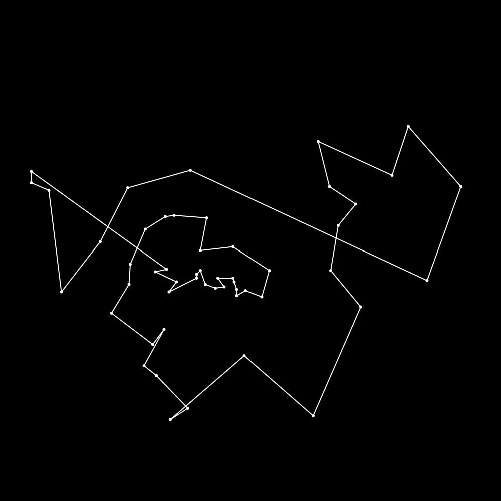
It's relatively obvious that the tour above can't be optimal to us humans. The main point here is that it has crossing edges which can never be part of the shortest path as "swapping" them as in the below animation always makes the path shorter.

Finding out which edges are crossing is not as easy for the computer as it is for us humans so in the so called 2-opt algorithm that we use the idea is to simply go through all possible pairs of edges swap them in the following way.

If we have two edges (A,B) and (C,D) and we do a two opt swap they will change to (A,C) and (B,D).

The new route cost of this new tour is computed and if it's shorter than the tour before we change to the new tour and start the 2-opt search again. It will be quite expensive to compute the tour cost from scratch each time. Fortunately the only thing that changes for a symmetric TSP are those two edges and the other edges stay the same or reverse their direction but keep the same cost.

This makes this heuristic relatively easy to implement, fast and is also quite effective.

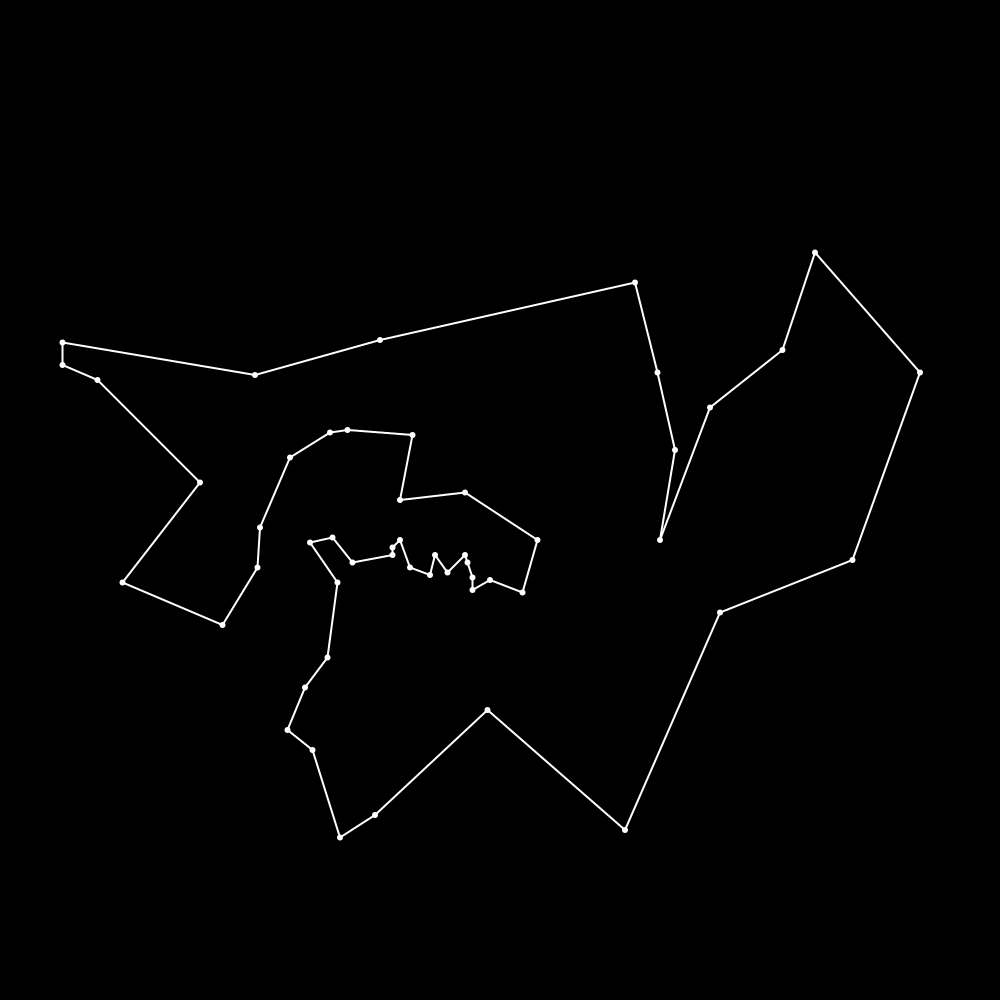
This tour already looks much better than the one before and brings us to a gap of 5.5% to the lower bound.

Reducing the memory consumption

Last time we have seen that our memory consumption is quite a big higher than that of TravelingSalesmanExact.jl

julia> @benchmark bnb_model = TSPSolver.optimize(joinpath(module_path, "../test/data/berlin52.tsp"))
BenchmarkTools.Trial: 13 samples with 1 evaluation.
 Range (min … max):  394.385 ms … 421.570 ms  ┊ GC (min … max): 7.74% … 10.08%
 Time  (median):     406.340 ms               ┊ GC (median):    8.62%
 Time  (mean ± σ):   406.939 ms ±   7.114 ms  ┊ GC (mean ± σ):  8.56% ±  0.78%

  ▁           ▁  ▁  ▁    ▁  █  █▁            ▁    ▁           ▁  
  █▁▁▁▁▁▁▁▁▁▁▁█▁▁█▁▁█▁▁▁▁█▁▁█▁▁██▁▁▁▁▁▁▁▁▁▁▁▁█▁▁▁▁█▁▁▁▁▁▁▁▁▁▁▁█ ▁
  394 ms           Histogram: frequency by time          422 ms <

 Memory estimate: 586.61 MiB, allocs estimate: 1734393.

julia> @benchmark tour, cost = get_optimal_tour(cities)
BenchmarkTools.Trial: 82 samples with 1 evaluation.
 Range (min … max):  52.062 ms … 77.058 ms  ┊ GC (min … max): 0.00% … 9.20%
 Time  (median):     58.953 ms              ┊ GC (median):    0.00%
 Time  (mean ± σ):   61.294 ms ±  5.591 ms  ┊ GC (mean ± σ):  1.58% ± 3.50%

           ▂    ▂█                  ▂                          
  ▅▄▁▁▁▁▄▄▅█▄▇▅▄████▁▅▄▁▁▄▄▁▇▄▅▁▁█▅▄█▄▅▄▄▁▄▄▄▅▁▁▄▁▁▁▁▄▁▄▄▅▁▁▄ ▁
  52.1 ms         Histogram: frequency by time        74.2 ms <

 Memory estimate: 10.19 MiB, allocs estimate: 130481.

and the plan was to improve up on this as well. There are of course several factors that play into the memory situation like how many nodes do we actually need to explore which we limited due to our previous improvements. Nevertheless there was one obvious thing to work on. Currently we make a deep copy of the root before we evaluate it as we need to set the fixed and disallowed edges.

We can change this quite easily by using saving which edges had which cost that we reduce down to 0 now due to fixing them or that we remove.

fixed_costs = Vector{Tuple{Tuple{Int,Int},Float64}}()
disallowed_costs = Vector{Tuple{Tuple{Int,Int},Float64}}()
for fixed_edge in node.fixed_edges
    extra_cost = fix_edge!(root, fixed_edge)
    sum_extra_cost += extra_cost
    push!(fixed_costs, (fixed_edge, extra_cost))
end
for disallowed_edge in node.disallowed_edges
    cost = get_prop(root.g, disallowed_edge..., :weight)
    push!(disallowed_costs, (disallowed_edge, cost))
    disallow_edge!(root, disallowed_edge)
end

after the evaluation of the node we simply need to add them again.

Lower bound produces a tour

One last thing that I want to mention in this small post is the fact that sometimes the lower bound algorithm doesn't just produce a lower bound but actually a valid tour. We count the degree of each vertex in the optimized 1-tree code anyway so we can find out easily whether a tour was created and can save time to compute a greedy solution which has likely a worse bound.

That's it for today 😄 Thanks for reading and hope you've learned something new.

Oh yeah maybe I should show you the new benchmark results 😂

julia> @benchmark bnb_model = TSPSolver.optimize(joinpath(@__DIR__, "..", "data", "berlin52.tsp"))
BenchmarkTools.Trial: 84 samples with 1 evaluation.
 Range (min … max):  55.460 ms … 72.157 ms  ┊ GC (min … max): 8.60% … 8.72%
 Time  (median):     59.324 ms              ┊ GC (median):    9.02%
 Time  (mean ± σ):   60.127 ms ±  3.250 ms  ┊ GC (mean ± σ):  9.34% ± 1.17%

        ▅▂▂ ▅▂█  █ ▅▂▅ ▅                                       
  ▅▁▁██████████▅██████▅█▁▅▅██▁█▁▁▅██▁▅▅▅███▁▁▁▁▁▁▁▁▁▁▁▁▅▅▁▁▁█ ▁
  55.5 ms         Histogram: frequency by time        68.8 ms <

 Memory estimate: 93.62 MiB, allocs estimate: 203263.

We are very close in performance now for this individual instance unfortunately still not able to solve a bigger one that I mentioned in the very first post. The memory consumption is still about an order of magnitude higher so maybe we have some more to gain here.

Stay tuned!

As always please feel free to check out my code on GitHub TSPSolver .

Special thanks to my 10 patrons!

Special special thanks to my >4$ patrons. The ones I thought couldn't be found 😄

• Anonymous

• Gurvesh Sanghera

• Szymon Bęczkowski

• Håkan Kjellerstrand

• Colin Phillips

For a donation of a single dollar per month you get early access to these posts. Your support will increase the time I can spend on working on this blog.

There is also a special tier if you want to get some help for your own project. You can checkout my mentoring post if you're interested in that and feel free to write me an E-mail if you have questions: o.kroeger <at> opensourc.es

I'll keep you updated on Twitter opensourcesblog.

Want to be updated? Consider subscribing on Patreon for free